This section provides preprocessing code to prepare LiDAR and sample plot data for subsequent point cloud deep learning model development.
Note
Expert knowledge is critical when preparing data for deep learning workflows, since small artifacts or errors in the data can have large impacts on downstream model performance.
Relevant Resources
The complete preprocessed dataset can be downloaded here as an alternative to running this notebook.
If you wish to run the preprocessing, the original height-normalized ALS and sample plot data for this analysis can be downloaded from the NFIS:
This tutorial makes use of the lidR package to prepare LiDAR data for deep learning. LiDAR preprocessing can often be complex and is a critical step in an enhanced forest inventory workflow. However, it is not the focus of this workshop. For more detailed information about LiDAR preprocessing, see the lidR package tutorial.
Dataset Background
The Petawawa Research Forest (PRF) is the oldest research forest in Canada, established in 1918. It is a remote sensing supersite and is part of the GEO-TREES network. The PRF represents a rich collection of open access traditional forest inventory and remote sensing data, including multiple LiDAR and aerial imagery acquisitions in addition to a large history of field plot measurements. These data are available at the National Forest Information System website. An article by White et al. (2019) summarizes the PRF in greater detail.
In this workshop, we make use of enhanced forest inventory sample plots collected in the PRF in 2018. We are also using single photon airborne laser scanning (ALS) data also collected in 2018.
Key information about the dataset
Sample plots are fixed-area and have a 14.1 m radius (625 m2).
Dataset size: n = 249 plots
Live trees with DBH > 9 cm measured (DBH, height, species, etc.)
ALS data has a mean point density of 35 points/m2.
Summary of Preprocessing Steps
LiDAR preprocessing
Examine and clean sample plot data
Determine dominant species type (coniferous/deciduous/mixed)
Derive plot-level total aboveground biomass (AGB) using allometry
Divide the data into training, validation, and test sets (i.e., splits)
Perform Z-score normalization for AGB data
Export preprocessed data
Filepaths
Ensure that the data is downloaded from here and that the filepaths below are correct prior to running any code.
Currently, the variable PROCESS_LIDAR is set to FALSE, which skips the LiDAR preprocessing code to save time. The preprocessed point cloud data is already provided in the dataset downloaded from the link above. However, if you wish to preprocess the ALS data, you can download the full Petawawa ALS dataset here.
Code
PROCESS_LIDAR =FALSEPLOT_RADIUS =14.1PLOT_COORDS_FPATH ='data/petawawa/SPL2018_EFI_ground_plots/SPL2018_EFI_ground_plots/PRF_SPL2018_EFI_plots_pts_wgs84.shp'PLOT_DATA_FPATH ='data/petawawa/SPL2018_EFI_ground_plots/SPL2018_EFI_ground_plots/PRF_CNL_SPL_CalibrationData_LiveDeadStems.xlsx'TREE_SP_CODES_FPATH ='data/petawawa/mnrf_sp_codes.csv'PLOT_PC_DIR ="data/petawawa/plot_point_clouds"PLOT_LAS_DIR ="data/petawawa/plot_las_files"LABELS_FPATH ='data/petawawa/labels.csv'ZQ95_FPATH ='data/petawawa/zq95.csv'LIDAR_INDEX_FPATH ='data/petawawa/prf_lidar_index.gpkg'ALLOMETRIC_FPATH ='data/petawawa/ung_lambert_allometric_dbh_eqs.csv'LIDAR_DIR =NA# The full ALS dataset is optional as preprocessed point clouds are provided (see above)
Packages
Ensure the following package dependencies are installed. Note that reticulate is an R package that allows for interfacing between R and Python languages. To use reticulate in this case, you need to have a Python virtual environment set up beforehand. Python environment setup instructions are provided here. Ensure that the data and Python environment are all stored in the same root directory as the tutorial files.
Code
library(lidR)library(here)library(sf)library(tidyverse)library(mapview)library(ggplot2)library(plotly)library(reticulate)library(readxl)library(purrr)library(DT)# Import Python numpy module using reticulatenp <- reticulate::import("numpy")
Study Area
We can start by examining the study area, including vector data representing ALS coverage of the PRF (i.e., the LiDAR index) and ground sample plot locations.
The plot data in this case were sampled in 2018 as a remeasurement of Temporary Sample Plots (TSP) originally established in 2013-2014 in support of an earlier LiDAR acquisition project.
The ALS data was collected in 2018 to support an EFI of the research forest.
Code
lidar_index <-st_read(LIDAR_INDEX_FPATH, quiet=TRUE)#Read the plot coordinates and ensure CRS is correctplot_centers <-st_read(here(PLOT_COORDS_FPATH), quiet=TRUE) %>%st_transform(st_crs(lidar_index)) %>%st_zm() %>% dplyr::rename(plot_id = Plot)mapview(lidar_index, layer.name ='LiDAR Tiles', map.types =c('Esri.WorldImagery'), alpha.regions =0.2, col.regions ='white', color ='grey') +mapview(plot_centers,col.regions ='red', color ='black', layer.name ='Ground Plots')
Code
# Helper function for viewing tabular dataview_table <-function(df){ DT::datatable(df, options =list(pageLength =5,columnDefs =list(list(className ='dt-center', targets ="_all"))),class ='cell-border stripe')}
1) LiDAR Preprocessing
Differences between conventional and deep learning ALS preprocessing for EFI
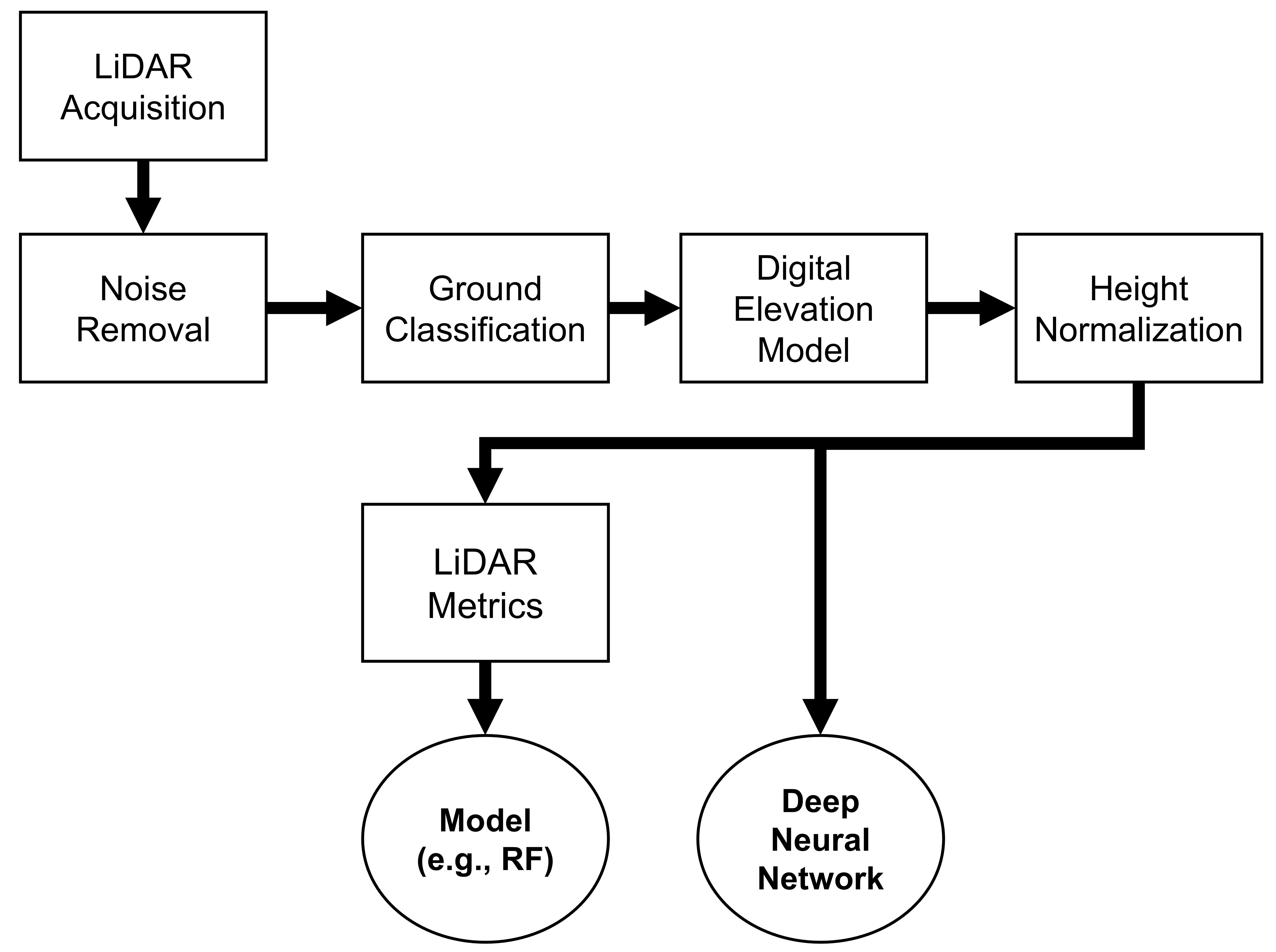
The flowchart below summarizes the ALS preprocessing pipeline to prepare data for EFI modelling using conventional and deep learning approaches. At the end of the flowchart, the key difference between the two approaches is the lack of LiDAR metric derivation.
Steps and Functions
The code below includes the LiDAR preprocessing steps to prepare the ALS point cloud data for use in deep neural network model development.
Most of these preprocessing steps are standard in any ALS - forest inventory workflow and are described in greater detail in the lidR package documentation. The steps are implemented as functions below, which are applied to each individual plot-level point cloud extracted from the full LiDAR acquisition. These steps include:
Extract and clean ALS point clouds contained within the boundary of the ground reference plots. We do this using the function extract_pc in the code below.
Filter duplicates, then classify and remove noisy points. This is performed using various functions from the lidR package combined in the clean_pc function.
Beyond this point, we abandon the LAS object from the lidR package and convert the point cloud to a simpler 3D array using the pc_to_matrix function. We do this because storing data in a simpler array format allows for faster reading time for deep learning model training.
We then normalize the point cloud data such that the X and Y coordinates are (0,0) at the center of the point cloud. This step improves deep neural network training outcomes as was outlined in early research by Qi et al. (2017). This is performed using the normalize_pc_xy function. Note that the Z coordinates are left as height above ground in meters.
We calculate the 95th height percentile for each plot point cloud for later comparison to ensure that there is good alignment between plot-level canopy height measurements and LiDAR height. We do this with the calc_pc_zq95 function.
Export point clouds to numpy files (.npy) for later use in model development using the write_pc_to_npy function. Note that other file formats (e.g., pickle, LAS, HDF5, PLY, etc.) are also used in point cloud deep learning applications. The choice of file format is case dependent. Here we favour the .npy format since it is fast and easy to work with in Python.
Here we apply the functions defined above to each individual sample plot point cloud.
Load a LAS Catalog representing the LiDAR data spanning the PRF.
Extract the corresponding point cloud for each plot with extract_pc
Clean the point clouds with clean_pc
Export the cleaned point clouds to LAS files (for use in random forest modelling)
Convert point clouds to arrays and normalize using pc_to_matrix and normalize_pc_xy
Calculate the 95th height percentile using calc_pc_zq95
Export the numpy point cloud files and the 95th height percentile data.
Code
if(PROCESS_LIDAR){#Read the normalized las catalog ctg <-readLAScatalog(LIDAR_DIR)#Set some catalog processing parametersopt_select(ctg) <-"xyz"opt_progress(ctg) <-FALSE# Ensure coordinate systems match plot_centers <- plot_centers %>%st_transform(lidR::crs(ctg))# Get a list of plot coordinates coords <-split(st_coordinates(plot_centers), seq_len(nrow(plot_centers)))# Extract point clouds and store in list las_ls <- purrr::map(coords, extract_pc, ctg = ctg, .progress =TRUE)# Clean point clouds las_ls <- purrr::map(las_ls, clean_pc, .progress =TRUE)# Ensure the LAS dir existsdir.create(PLOT_LAS_DIR, recursive =TRUE, showWarnings =FALSE)# Export cleaned las filesfor(i in1:nrow(plot_centers)){ plot_id <- plot_centers$plot_id[i] las_fpath <-here(file.path(PLOT_LAS_DIR, paste0(plot_id, ".las"))) lidR::writeLAS(las_ls[[i]], las_fpath) }# Convert point clouds to matrices pc_ls <- purrr::map(las_ls, pc_to_matrix, .progress =TRUE)# Normalize point clouds X & Y coordinates (leave Z) pc_ls <- purrr::map(pc_ls, normalize_pc_xy, .progress =TRUE)# Calculate zq95 for each point cloud to check alignment with plot data later als_derived_zq95_ls <- purrr::map(pc_ls, calc_pc_zq95, .progress =TRUE)# Ensure the point cloud directory existsdir.create(PLOT_PC_DIR, recursive =TRUE, showWarnings =FALSE)# Export point clouds to numpy (.npy) files for use in Pythonmapply(write_pc_to_npy, pc = pc_ls,plot_id = plot_centers$plot_id,pc_out_dir=PLOT_PC_DIR)# Export ZQ95 values als_derived_zq95_df <-data.frame(plot_id = plot_centers$plot_id,als_zq95 =as.numeric(als_derived_zq95_ls))write.csv(als_derived_zq95_df, ZQ95_FPATH, row.names=FALSE)}
Preprocessed point cloud example
The plot below shows the point cloud for a plot in the PRF dataset. Note that the X and Y coordinates are now normalized and are relative to the plot center.
Code
plot_pc <-function(pc){ pc_df <-as.data.frame(pc)names(pc_df) <-c('x', 'y', 'z') p <-plot_ly(pc_df, x =~x, y =~y, z =~z, type ="scatter3d", mode ="markers",marker =list(size =3, color =~z, colorscale ="Jet")) %>%layout(title ="",scene =list(xaxis =list(title ="", showgrid =FALSE, showticklabels =TRUE, ticks ="outside"),yaxis =list(title ="", showgrid =FALSE, showticklabels =TRUE, ticks ="outside"),zaxis =list(title ="Z", showgrid =FALSE, showticklabels =TRUE, ticks ="outside") ))return(p)}# Load an example pcdemo_pc <- np$load(list.files(PLOT_PC_DIR, full.names =TRUE)[50])# Visualize a point cloudplot_pc(demo_pc)
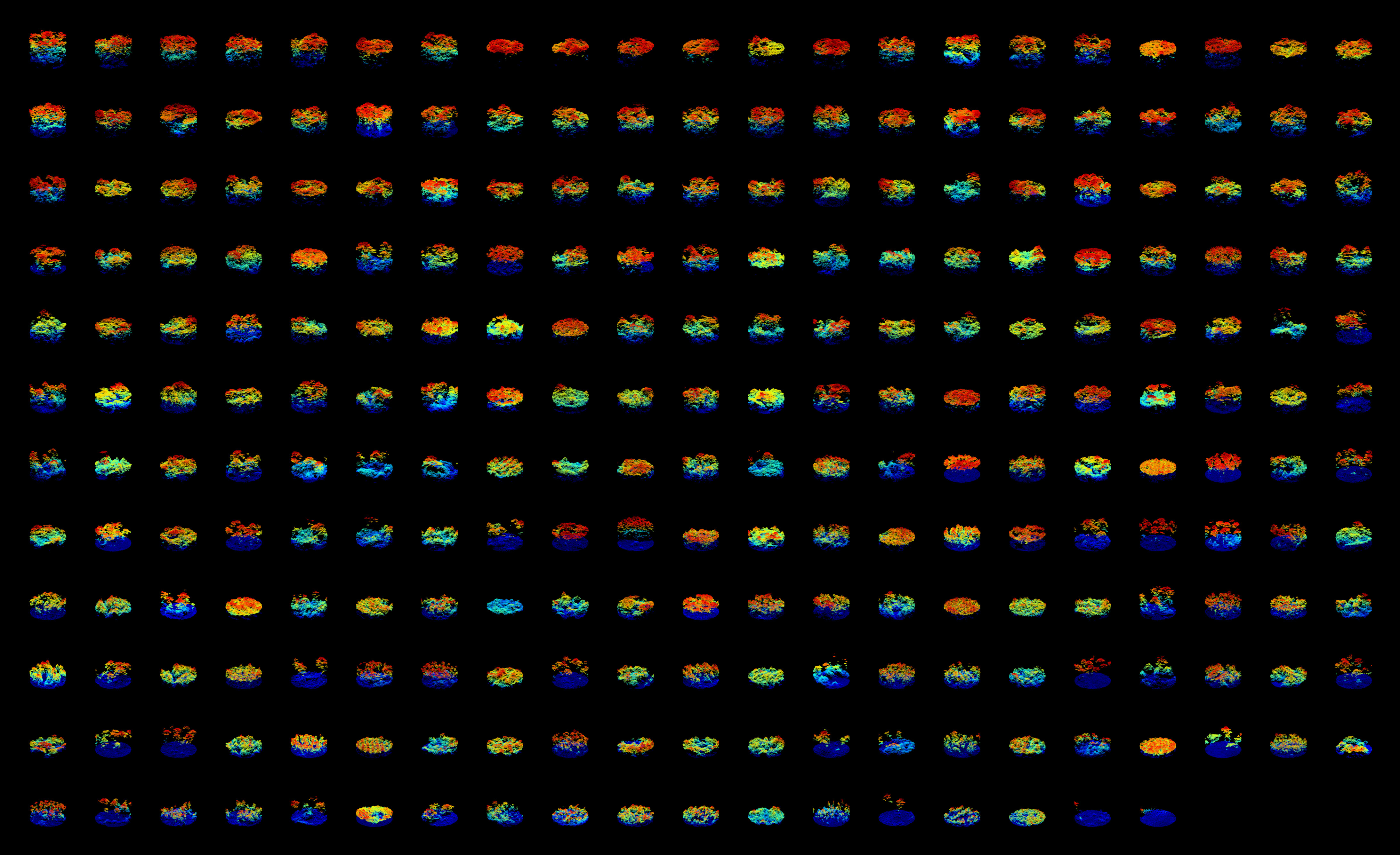
Preprocessed point clouds
The image below shows the 249 sample plot point clouds in the PRF from 2018. Plots are listed in decreasing order based on canopy height. Click the image to view in full screen.
2) Prepare Sample Plot Data
We now move on to loading and examining the tree-level measurements across the PRF sample plots (n = 249).
Below we perform the following:
Load tree species codes to get the full names for subsequent joining with allometric equation parameters.
Load individual tree measurements from the PRF_CNL_SPL_CalibrationData_LiveDeadStems.xlsx spreadsheet.
Remove any dead stems from the tree list and join the data with the species names
Below we load tree-level measurements and inspect the data
Code
# Load tree species codestree_sp_codes_df <-read.csv(TREE_SP_CODES_FPATH) %>%mutate(species =trimws(species))# Load plot level tree measurementstrees_df <-read_excel(PLOT_DATA_FPATH, sheet ='Tree') %>% dplyr::rename(plot_id = PlotName,sp_code = tree_spec,dbh = DBH) %>%select(plot_id, sp_code, dbh, ht_meas, tvol, Status) %>%# Drop dead trees from datasetfilter(Status =="L") %>%# Add species names from codes dfleft_join(tree_sp_codes_df, by ='sp_code') %>%#Capitalize species namemutate(species =str_to_title(species))# View the first 30 trees in the datasettrees_df %>%head(30) %>%view_table()
Examine species composition
Below we check for missing species data and summarize the overall species composition in the dataset based on count.
# Check for NAsstopifnot(all(!is.na(trees_df$species)))# Sort by decreasing species occurrence based on counttrees_df %>%count(species) %>%mutate(percent =round(n /sum(n) *100, 2)) %>%arrange(desc(percent)) %>%mutate(across(where(is.numeric), ~round(.x, 1))) %>%rename(Species=species,`N Trees`=n,`Percent of Total Trees (%)`=percent) %>%view_table()
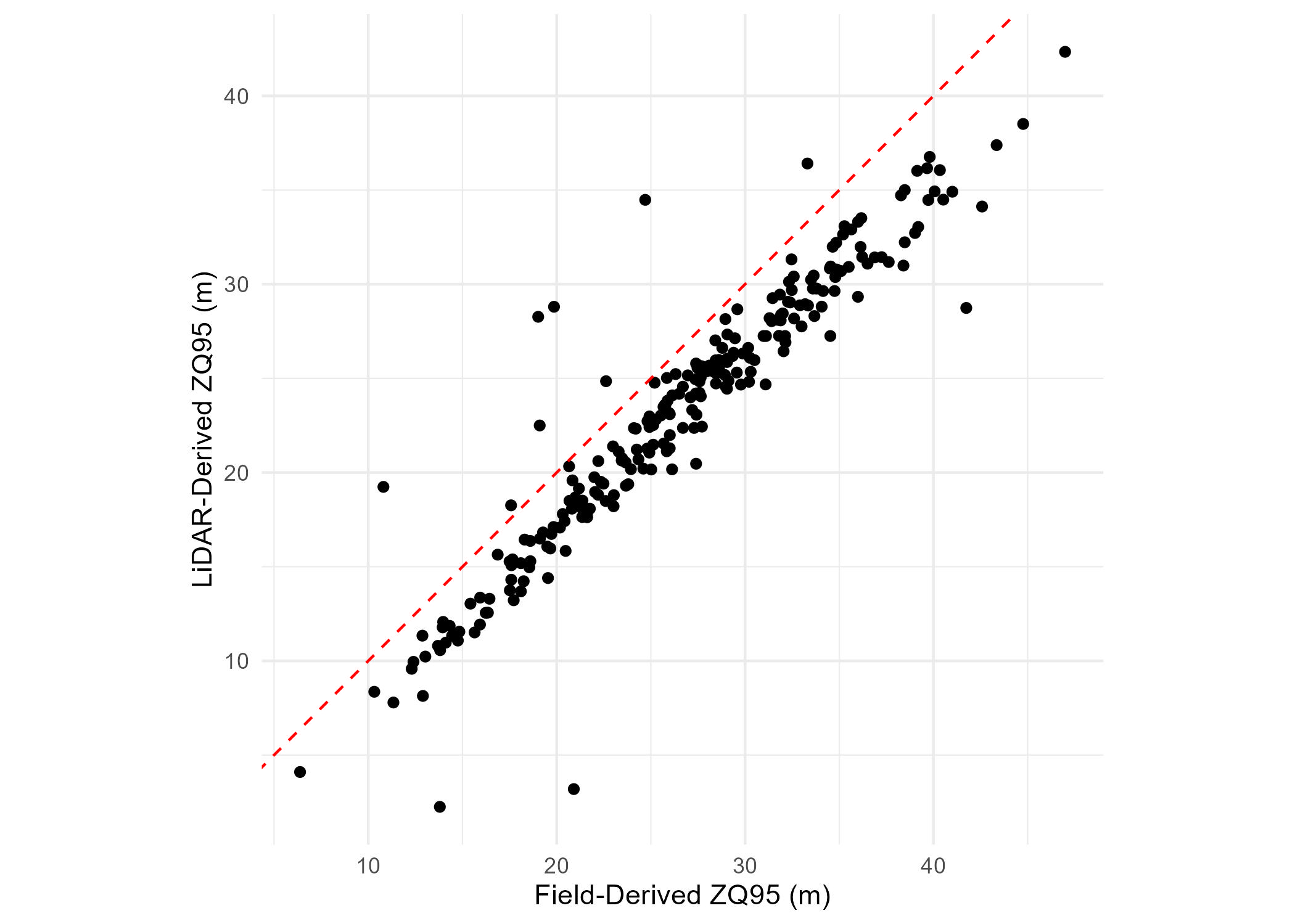
Check alignment between LiDAR and plot data
An effective way to check the alignment between the preprocessed LiDAR and plot data is by comparing plot-level canopy height measurements with LiDAR-derived 95th height percentile. If there is a strong correlation, this indicates good alignment.
Below we perform the following:
Load the previously derived LiDAR-derived 95th height percentile values (ZQ95)
Derive plot-level ZQ95 based on field tree height measurements.
Visualize the field-derived ZQ95 vs. the LiDAR-derived ZQ95.
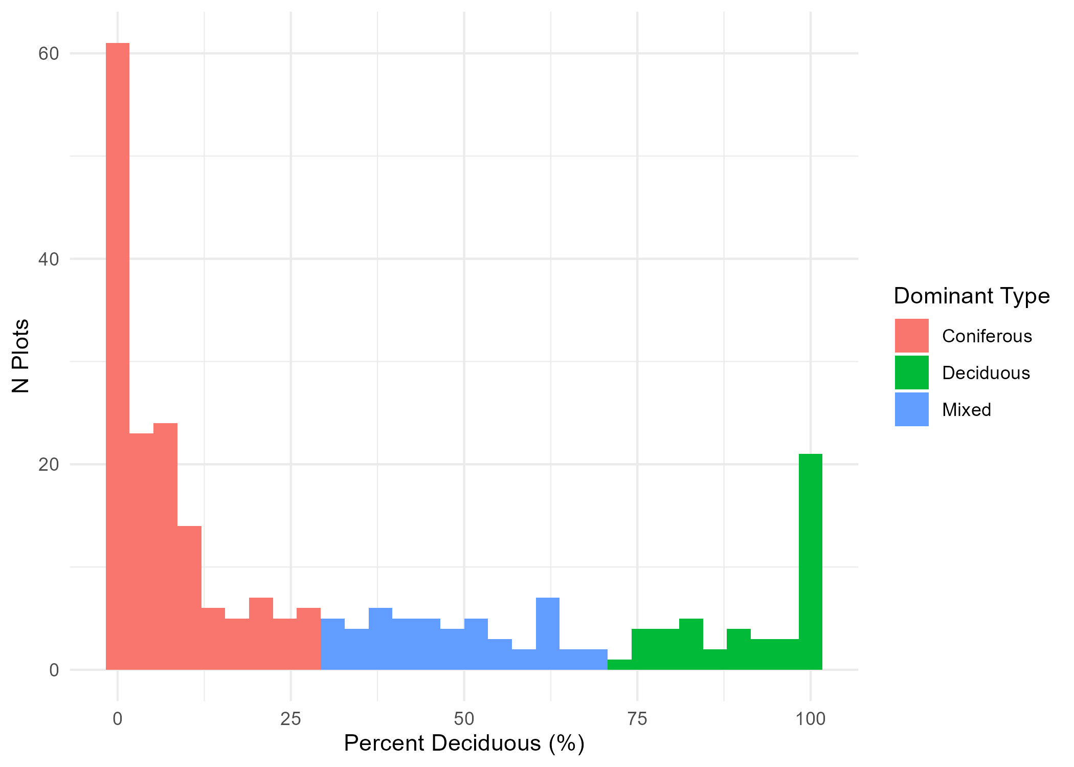
Here we classify each plot as dominated by coniferous, deciduous, or mixed. These three classes will later be used to train a deep neural network classifier in the TRAIN section of the tutorial.
For the purpose of this tutorial, we will use total volume (tvol) derived from field plot tree measurements to define species dominance.
In the code below we do the following:
Set a volume percentage threshold to define species dominance (DOMINANCE_PERC_THRESH).
Define a function (get_tvol_d_perc) to derive the plot total volume (plot_tvol) and the total deciduous volume (decid_tvol). We then use both of these to derive the percentage of deciduous volume comprising each plot.
We apply the get_tvol_d_perc to each plot and use the DOMINANCE_PERC_THRESH to assign a plot to either coniferous, deciduous, or mixed using the following logic:
Note that for the purpose of this tutorial, we use the DBH-only allometric equations since not all trees in the field data have height measurements.
In the code below we:
Load the allometric equation parameters from Lambert et al. (2005)
Fix issues with species names to match those in the allometric data
Check that all species names match
allo_eqs_fpath =here(ALLOMETRIC_FPATH)allo_df <-read.csv(allo_eqs_fpath) %>%rename(species = Species_en) %>%mutate(species =str_to_title(species))allo_sp_nms <-sort(unique(allo_df$species))# Rename species to match allometric names# Red (Soft) Maple as Red Mapletrees_df$species[trees_df$species =="Red (Soft) Maple"] <-"Red Maple"# Ironwood (Ostrya virginiana) as Hop-Hornbeamtrees_df$species[trees_df$species =="Ironwood"] <-"Hop-Hornbeam"# Tamarack as Tamarack Larchtrees_df$species[trees_df$species =="Tamarack"] <-"Tamarack Larch"# White pine as Eastern white pinetrees_df$species[trees_df$species =="White Pine"] <-"Eastern White Pine"# American Elm as White elmtrees_df$species[trees_df$species =="American Elm"] <-"White Elm"#Northern White Cedar as Eastern white cedartrees_df$species[trees_df$species =="Northern White Cedar"] <-"Eastern White Cedar"#Check that all species names in data correspond to those in allometric eqsstopifnot(all(unique(trees_df$species) %in%unique(allo_df$species)))
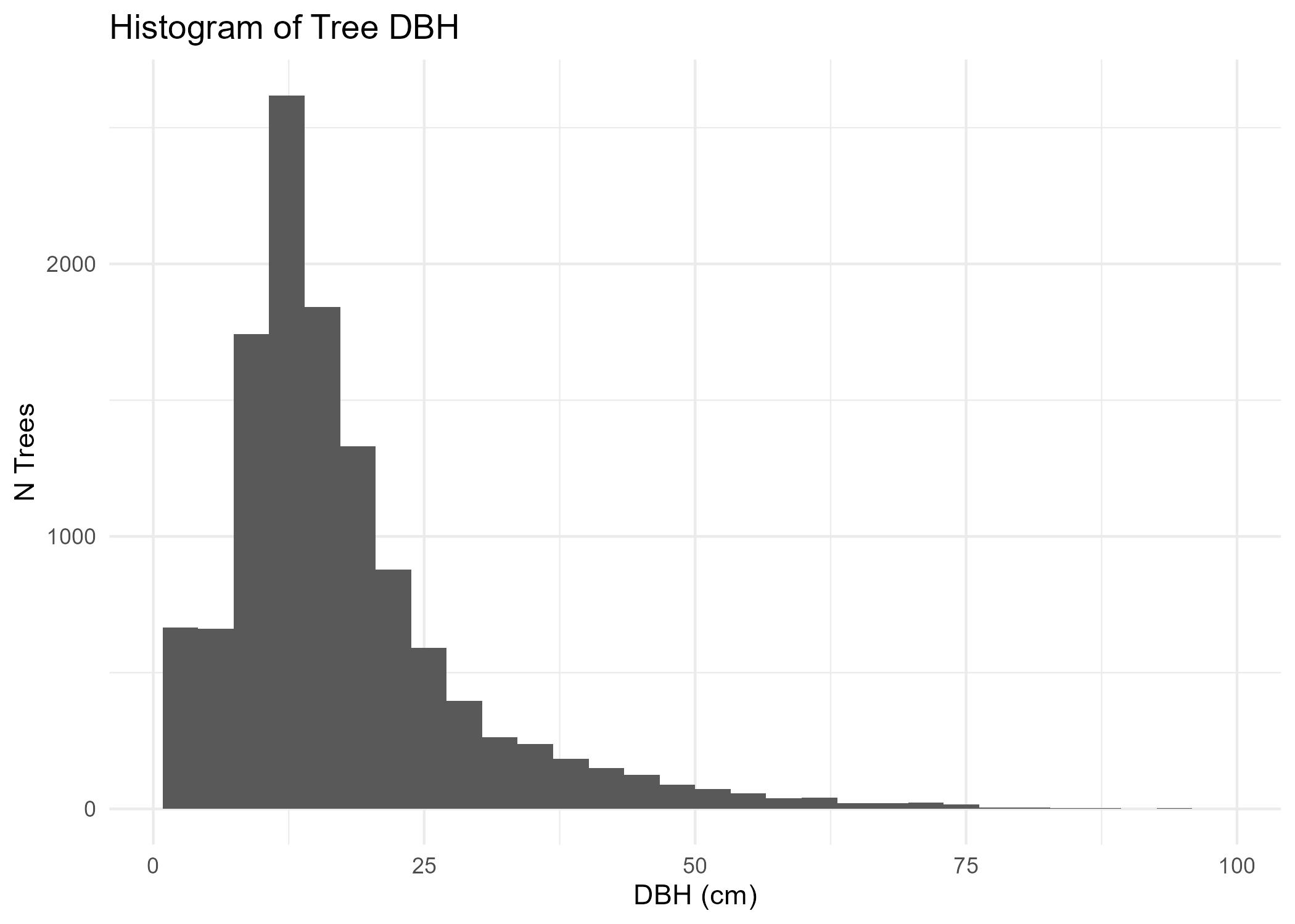
Check distribution of DBH values
Code
fig <- trees_df %>%ggplot(aes(x = dbh)) +geom_histogram() +ggtitle("Histogram of Tree DBH") +theme_minimal() +xlab("DBH (cm)") +ylab('N Trees')ggsave(filename =here('images/trees_dbh_histogram.jpg'),plot = fig)
In the code below, we pivot the allometric data frame to a wide format for easier implementation
Code
# Pivot allometric equations to wide formatallo_df_wide <- allo_df %>%select(species, Component_en, a, b) %>%pivot_wider(names_from = Component_en, values_from =c(a, b))view_table(allo_df_wide)
Define functions to calculate AGB for each tree
Code
get_biomass <-function(a, b, c, dbh){ #DBH in cm, height in meters Biomass_kg <- a * (dbh^b)return(Biomass_kg)}get_tree_comp_biomass <-function(tree_df, use_height=FALSE){ tree_df['foliage_biomass_kg'] <-get_biomass(a=tree_df['a_Foliage'], b=tree_df['b_Foliage'], c=tree_df['c_Foliage'],dbh=tree_df['dbh']) tree_df['bark_biomass_kg'] <-get_biomass(a=tree_df['a_Bark'], b=tree_df['b_Bark'], c=tree_df['c_Bark'],dbh=tree_df['dbh']) tree_df['branches_biomass_kg'] <-get_biomass(a=tree_df['a_Branches'], b=tree_df['b_Branches'], c=tree_df['c_Branches'],dbh=tree_df['dbh']) tree_df['wood_biomass_kg'] <-get_biomass(a=tree_df['a_Wood'], b=tree_df['b_Wood'], c=tree_df['c_Wood'],dbh=tree_df['dbh'])return(tree_df)}
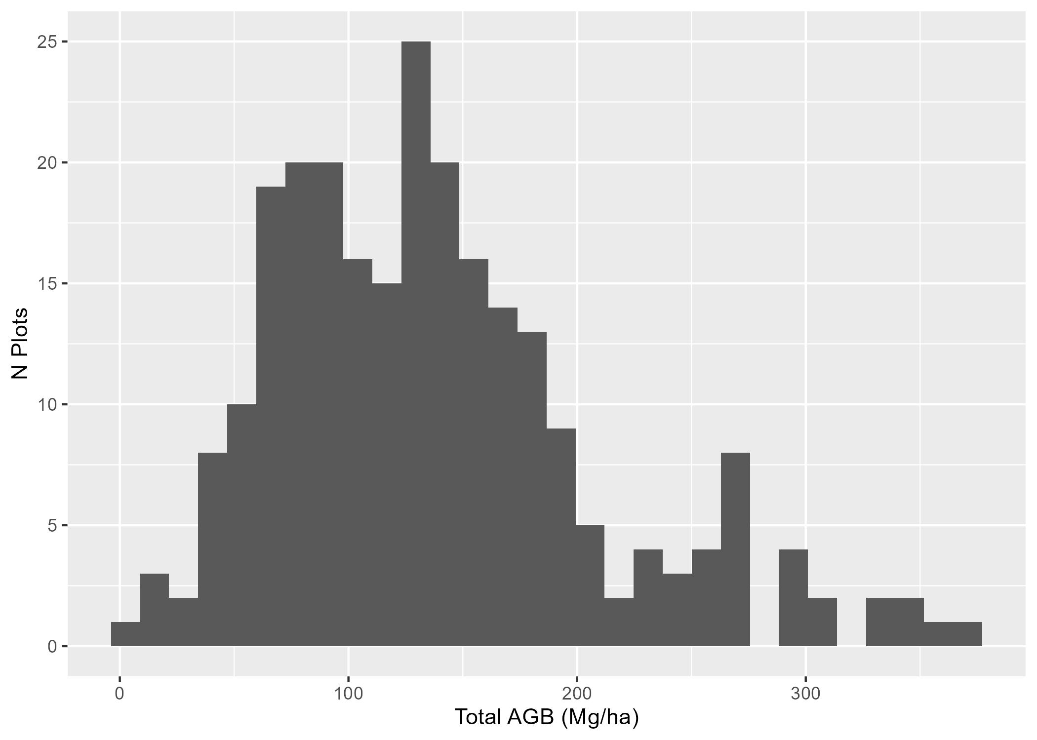
Derive tree-level and subsequently plot-level AGB
Here we take the following steps to derive plot-level AGB:
Join the trees with allometric parameters based on species name
Apply the get_tree_comp_biomass to calculate tree component biomass (Foliage, Bark, Branch, Wood)
Sum tree biomass components to get total_biomass_kg in kilograms (kg) for each tree
Sum tree AGB for each plot to get plot-level AGB (total_agb_kg)
Convert to tonnes per hectare (Mg/ha) using the plot area in hectares (0.06246 ha)
trees_agb_df <- trees_df %>%left_join(allo_df_wide, by ="species") %>%get_tree_comp_biomass(.) %>%mutate(total_biomass_kg = foliage_biomass_kg + bark_biomass_kg + branches_biomass_kg + wood_biomass_kg)# Check for NAsstopifnot(all(!is.na(trees_agb_df$total_biomass_kg)))# Each plot has a radius of 14.10m, so an area of 624.6m^2# 1m^2 == 0.0001 ha# So each plot is 0.06246 haplot_area_in_ha =0.06246#Summarize biomass by component for each plotbiomass_df <- trees_agb_df %>%group_by(plot_id) %>%summarise(total_agb_kg =sum(total_biomass_kg))# Divide by 1000 for tonnes conversion, then by plot area in ha to get tonnes/ha# 1t == 1000 kg, per hectarebiomass_df <- biomass_df %>%mutate(total_agb_mg_ha = total_agb_kg/1000/plot_area_in_ha)fig <- biomass_df %>%ggplot(aes(x = total_agb_mg_ha)) +geom_histogram() +xlab("Total AGB (Mg/ha)") +ylab("N Plots")ggsave(filename =here('images/agb_histogram.jpg'),plot = fig)
5) Split Datasets
In deep learning applications, there is a requirement for three different subsets of your dataset: training, validation, and test. These are referred to as dataset splits.
The Training split is used to fit the deep neural network to patterns in the data in order to predict the target.
The Validation split is used during model fitting iteratively to evaluate whether the model is generalizing well. Typically, model training is stopped when performance on the validation split is optimal.
The Test split is used for final model assessment. The test data is kept completely isolated during the model fitting process and is used at the end to evaluate how well the deep neural network generalizes to unseen data.
Below we combine the biomass and dominant species data
# Join species and biomass data framesdf <- perc_decid_df %>%left_join(biomass_df, by ='plot_id')# Check for NAsstopifnot(all(!is.na(df$total_agb_mg_ha)),all(!is.na(df$dom_sp_type)))
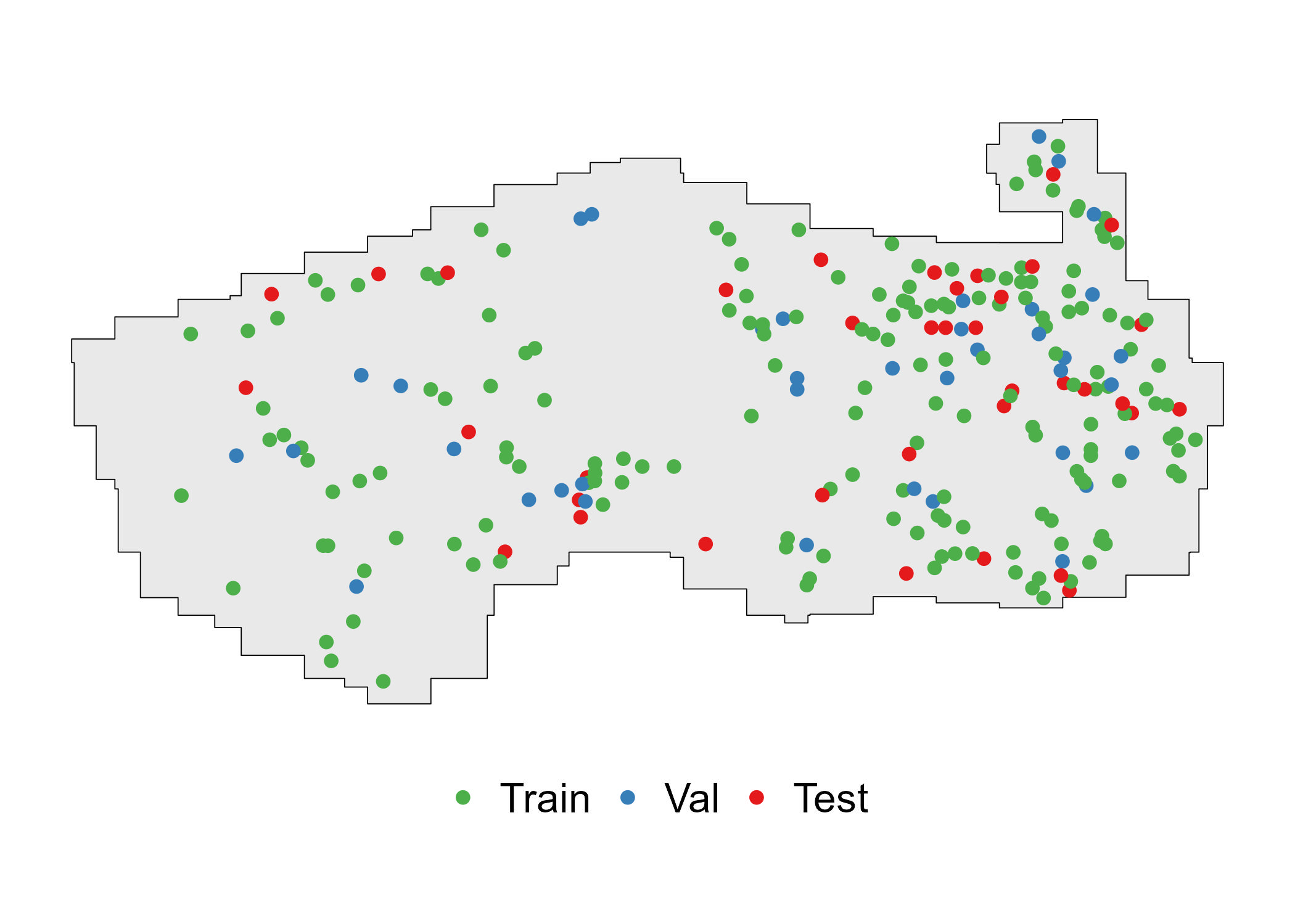
Divide data into training, validation, and testing
We randomly assign 70% of the plots to the train split, 15% to validation, and the remaining 15% to test.
Note
Note that in many cases, it is useful to divide samples into splits using a stratified sampling procedure based on the response variable. For the purpose of this tutorial, we will simply assign samples to each split randomly. However, note that for imbalanced datasets this may result in poor model performance, especially if the test split does not align well with the train split. As such, other strategies can be used to get better alignment between splits, such as stratified sampling or cross-validation.
train_prop <-0.7val_prop <-0.15test_prop <-0.15stopifnot(train_prop + val_prop + test_prop ==1)# Establish the number of samples per splitn_test <-round(nrow(df) *0.15, 0)n_train <-round(nrow(df) *0.70, 0)set.seed(14)test_df <- df %>%slice_sample(n=n_test) %>%mutate(split ="test")set.seed(14)train_df <- df %>%anti_join(test_df, by ="plot_id") %>%slice_sample(n=n_train) %>%mutate(split ="train")val_df <- df %>%anti_join(train_df, by ="plot_id") %>%anti_join(test_df, by ="plot_id") %>%mutate(split ="val")# Combine data frameslabels_df <- dplyr::bind_rows(train_df, val_df, test_df) %>%select(c(plot_id, dom_sp_type, perc_decid, total_agb_mg_ha, split)) %>%mutate(split =factor(split,levels =c('train', 'val', 'test'),ordered =TRUE))
Get a summary of the dataset splits:
Train: 174 plots (70%)
Validation: 38 plots (15%)
Test: 37 plots (15%)
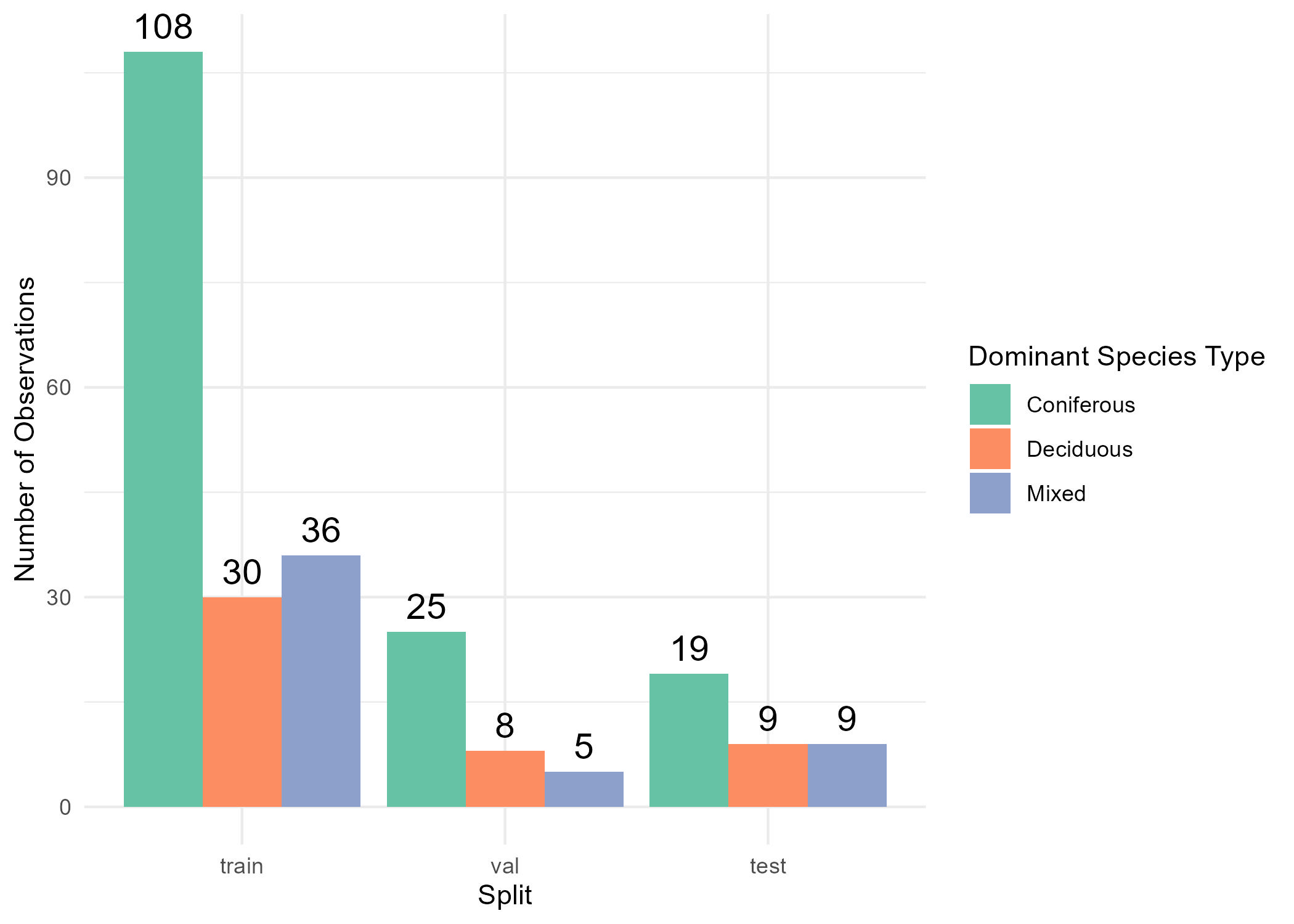
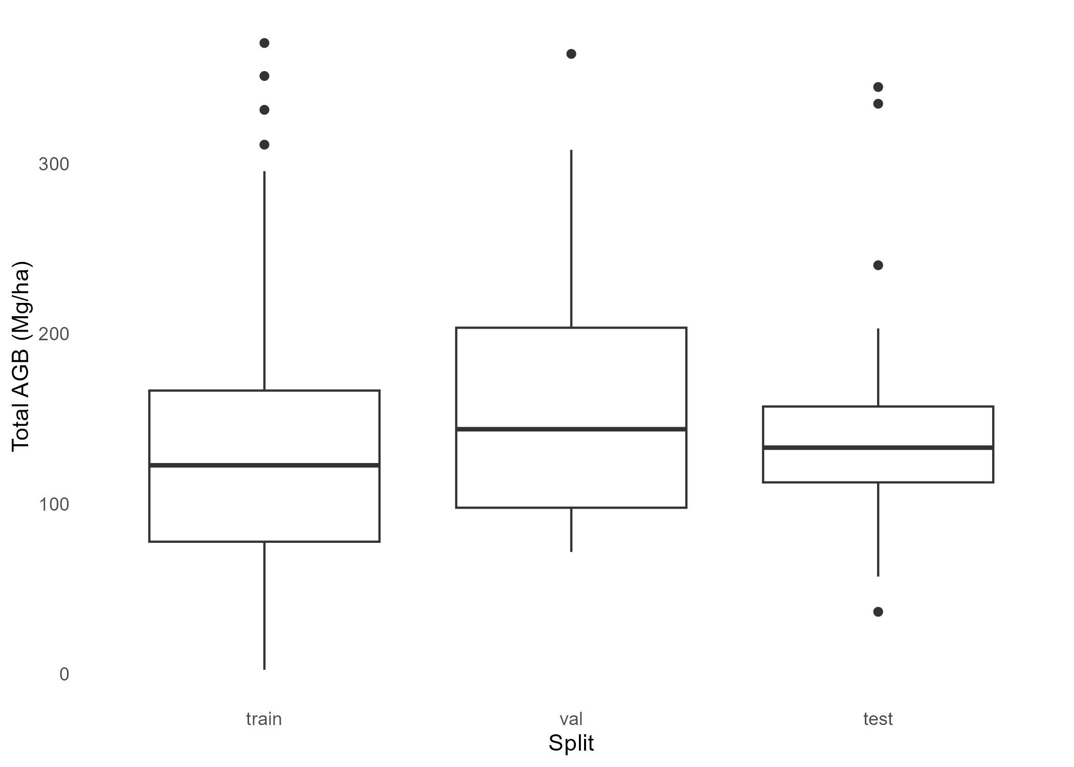
Examine the dominant species type and aboveground biomass labels with assigned dataset splits
# View species type frequency by splitfig1 <-ggplot(labels_df, aes(x = split, fill = dom_sp_type)) +geom_bar(position ="dodge") +geom_text(stat ="count", aes(label = ..count..), position =position_dodge(width =0.9), vjust =-0.5, color ="black", size =5) +labs(x ="Split",y ="Number of Observations",fill ="Dominant Species Type") +theme_minimal() +scale_fill_brewer(palette ="Set2",labels =c("conif"="Coniferous", "decid"="Deciduous", "mixed"="Mixed") )# View biomass variation by splitfig2 <- labels_df %>%ggplot(aes(x = split, y = total_agb_mg_ha)) +geom_boxplot() +theme_minimal() +theme(panel.grid =element_blank(), ) +xlab("Split") +ylab("Total AGB (Mg/ha)")# Export figuresggsave(filename =here('images/species_splits_barplot.jpg'), plot = fig1)ggsave(filename =here('images/total_agb_splits_boxplots.jpg'), plot = fig2)
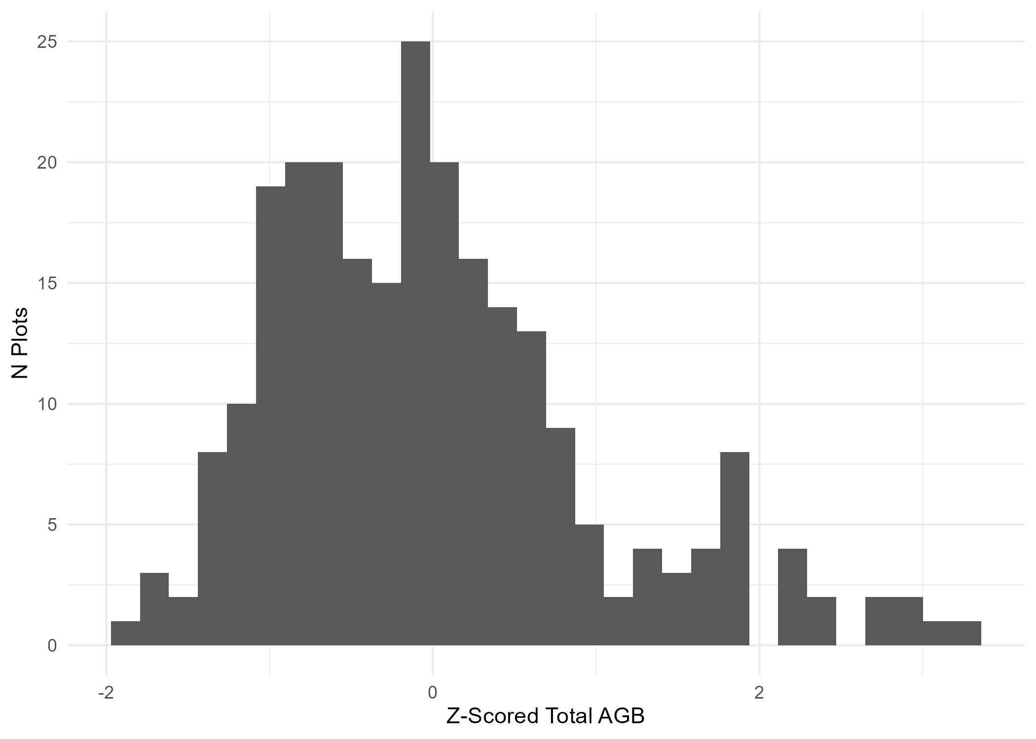
6) Z-score AGB
In many deep learning regression problems, response variables are z-score normalized to improve training stability. Here we z-score the AGB values as shown in the code and plot below.
We have finished preparing the LiDAR, dominant species, and biomass data for deep learning training. This yields the following in our data directory:
Sample plot point clouds stored as numpy array files (.npy) in data/petawawa/plot_point_clouds
Dominant tree species and aboveground biomass of each plot stored in data/petawawa/labels.csv
Code
# Ensure that labels correspond to existing point cloud filespc_flist <-list.files(PLOT_PC_DIR, full.names =TRUE)pc_id_ls <-gsub(".npy", "", basename(pc_flist))# Ensure labels contain the same plots as the ALS point cloudslabels_df <- labels_df %>%filter(plot_id %in% pc_id_ls)# Export labelswrite.csv(labels_df, LABELS_FPATH, row.names=FALSE)
Below we visualize an example point cloud with dominant species and biomass labels