Training Deep Learning Models

Relevant Resources

Below we provide references to additional materials relevant to this section.

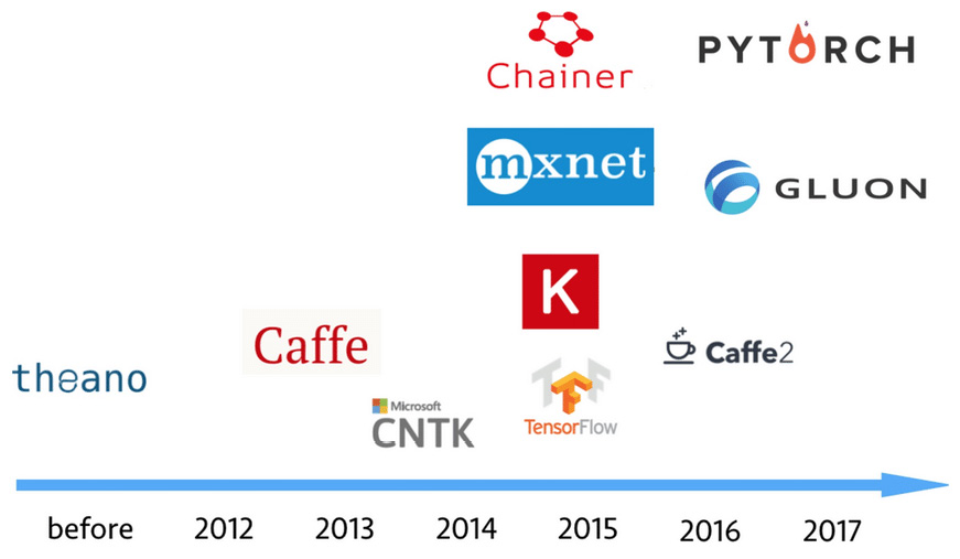
Other Deep Learning Frameworks

Introduction

Deep Neural Networks (DNNs), specifically those designed for 3D point clouds, are powerful tools for automation. This tutorial outlines how to use the PyTorch Lightning (PL) framework to train a specific and highly effective model—the Dynamic Graph CNN (DGCNN)—on your plot data.

Our goal is to automate complex analyses, such as:

Classification: Automatically determining the forest type (e.g., coniferous/deciduous/mixed) for a plot.
Regression: Estimating biomass or predicting tree attributes like total height or basal area.

Source code is available on GitHub

└── src
    ├── README.md
    ├── config.py
    ├── dataset
        ├── data_utils.py
        ├── efi_datamodule.py
        └── efi_dataset.py
    ├── models
        ├── dgcnn.py
        ├── efi_modelmodule.py
        ├── heads.py
        ├── loss_utils.py
        ├── metrics.py
        ├── pointnet.py
        ├── pointnet2_msg.py
        ├── pointnet2_ssg.py
        ├── pointnet2_utils.py
        ├── pointnet_utils.py
        └── pointnext.py
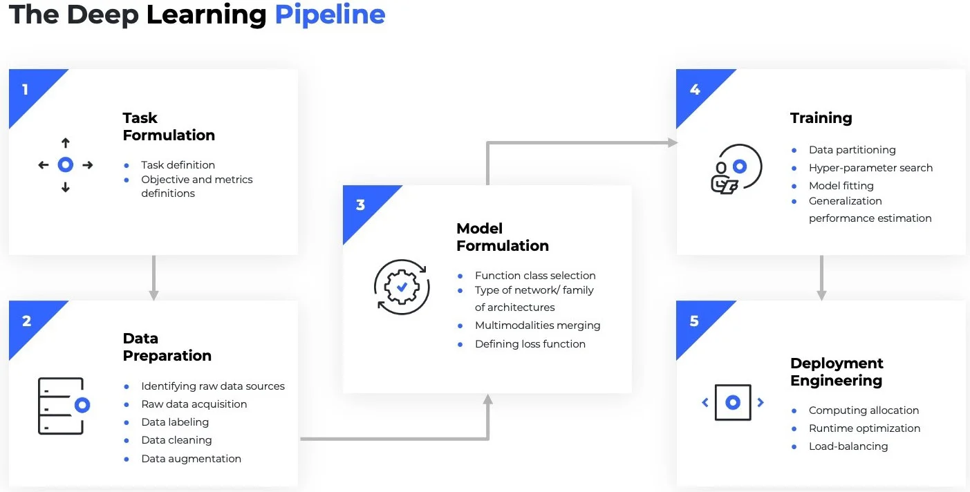
    └── train_pl.py

Deep Learning Pipeline

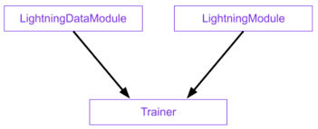
The Core Components of PyTorch Lightning:

LightningDataModule standardizes the training, val, test splits, data preparation and transforms. It takes in a custom PyTorch Dataset and DataLoader, which enables the Trainer to handle data during training. If needed, LightningDataModule exposes the setup and prepare_data functions in case you need additional customization.
LightningModule itself is a custom torch.nn.Module that is extended with dozens of additional functions like on_fit_start and on_fit_end. These functions allow us better control of Trainer’s flows and enable custom behaviors by overriding these hooks.
Trainer configures the training scope and manages the training loop with LightningModule and LightningDataModule. The simplest Trainer configuration is accomplished by setting flags like devices, accelerator, and strategy and by passing in our choice of loggers, profilers, callbacks, and plugins.

The Data Foundation: The EFI Point Cloud Dataset

The first step in any deep learning project is getting your data from files on disk into tensors on the GPU.

In this project, that job is handled by two Python scripts:

EfiDataset.py — reads and prepares individual plots
EfiDataModule.py — organizes those plots into training, validation, and test loaders

Tip

Tensor?

Tensors are the fundamental building block of deep learning. Their job is to represent data in a numerical way. An n-dimensional array of numbers, a 0-dimension tensor is a scalar, a 1-dimension tensor is a vector

The `EfiDataset` (efi_dataset.py)

The EfiDataset class defines how to read your raw point cloud files (e.g., .npy format saved for each plot) and your labels file (e.g., labels.csv in our workshop) for the model.

What it does

Reads raw files

Loads point clouds from .npy files
Reads labels from labels.csv (e.g., dom_sp_type for classification or total_agb_z for biomass regression)

Samples points

Selects a fixed number of points (num_point, default: 8192)
This keeps memory usage manageable and ensures every batch has the same shape

Computes optional features

Surface normals (local orientation of points)

Caches processed data

If --process_data is enabled, it saves a processed version to disk (_process_and_cache()). Future runs load this cached data instead of reprocessing (_load_cache()). This avoids resampling the raw data every time you train, drastically speeding up development. Else: on-the-fly.

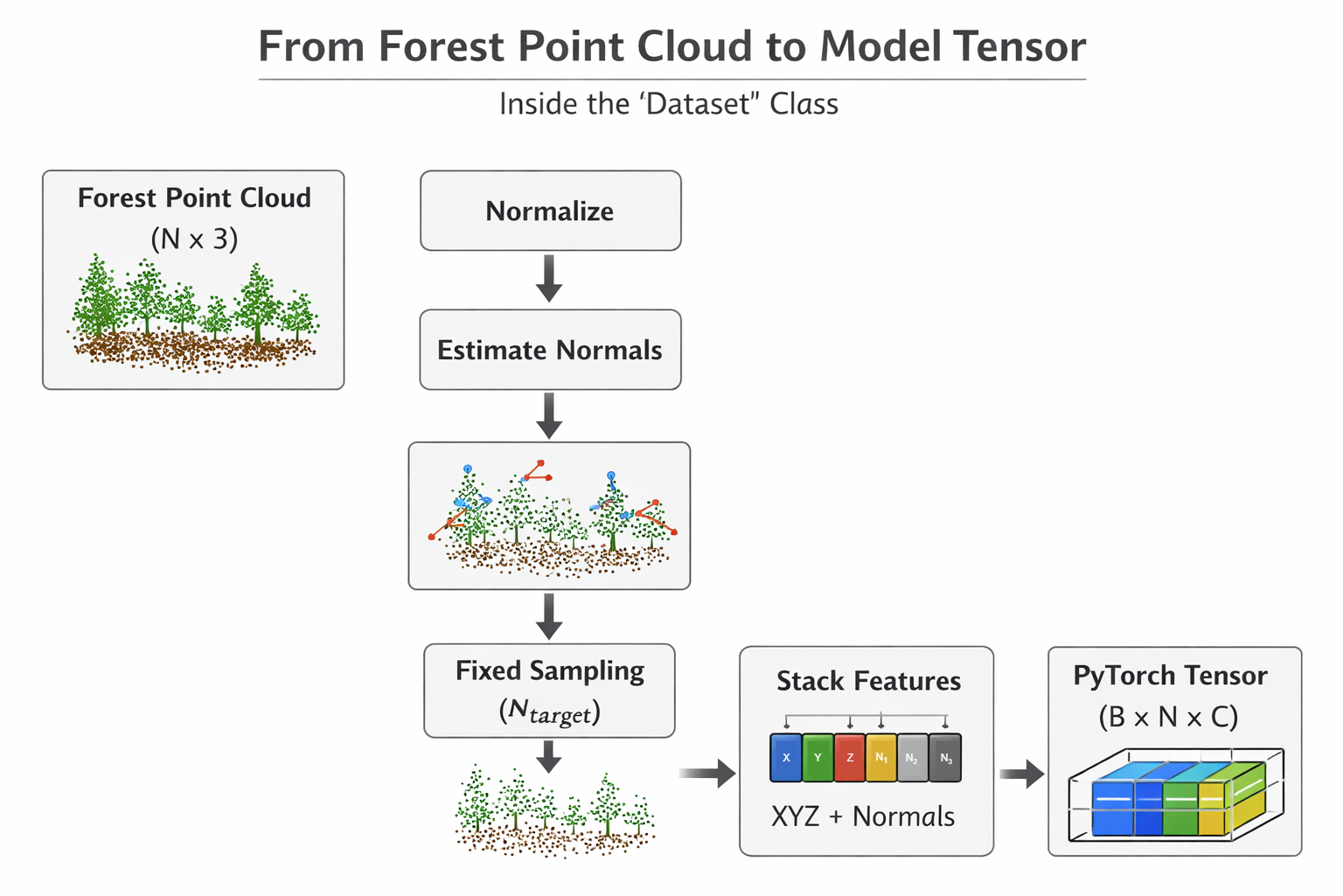
Figure 4: `EfiDataset` workflow (Generated by ChatGPT)

Why 8192? Point clouds are massive. We downsample to a fixed number so we can process them in batches. If we used the full points of a LiDAR plot, we’d run out of GPU memory instantly. 8192 is a typical ‘sweet spot’ for DNNs to retain structural information without crashing the hardware. We didn’t test all possible settings in our demo—try it out!

The `EfiDataModule` (efi_datamodule.py)

In the PyTorch Lightning framework, the EfiDataModule wraps the EfiDataset to handle the data workflow. It controls how plots move through the training system.

What it manages

Which plots go into:

The setup() function creates three datasets:

train_dataset
val_dataset
test_dataset

Each one uses the same loading logic, but different rows from the label file (e.g., using the split column in labels.csv).

How big each batch is
How many background workers load data in parallel (make sure batches are efficiently provided to the GPU workers).

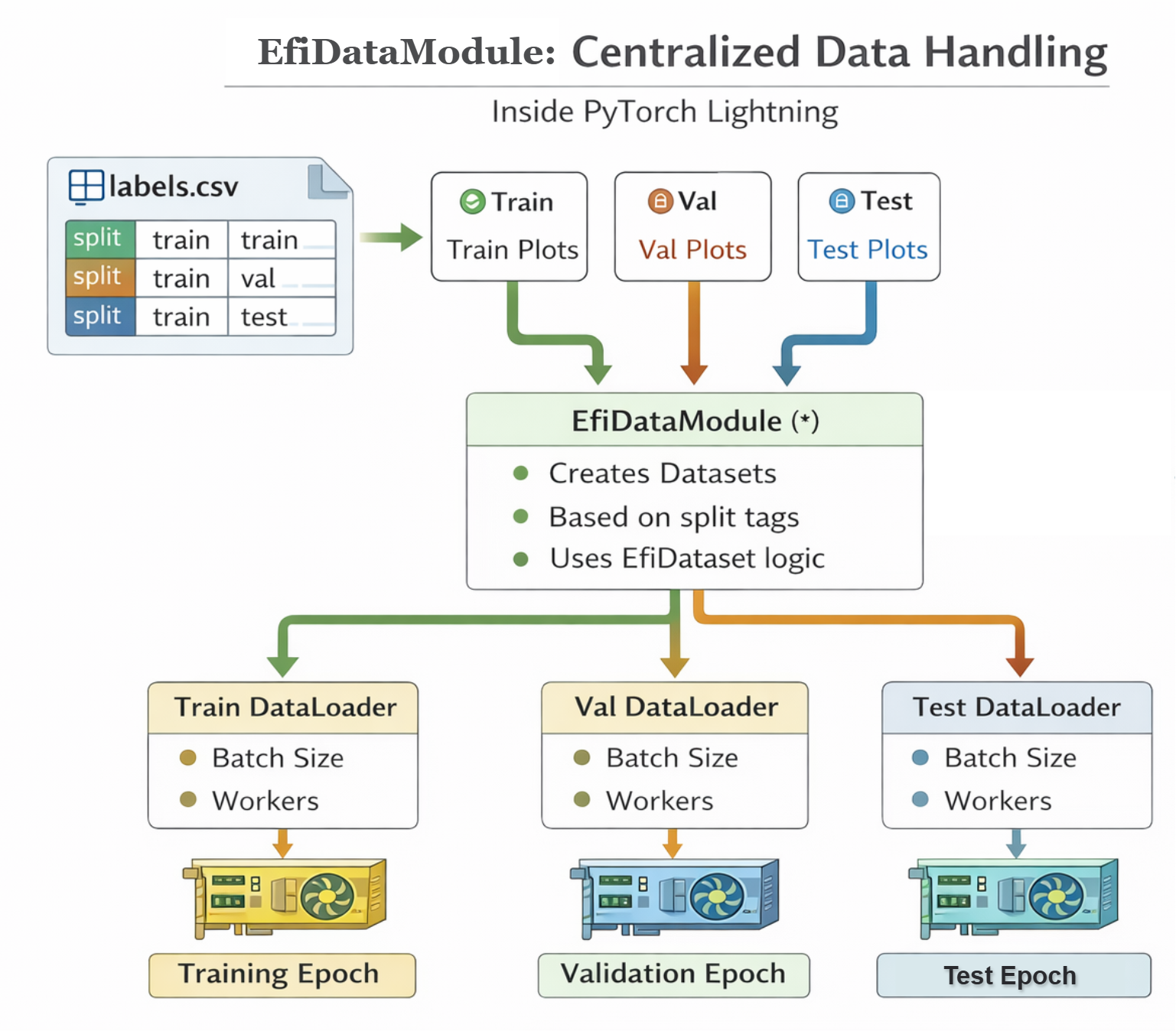
Figure 5: `EfiDataModule` workflow (Generated by ChatGPT)

# efi_datamodule.py
import pytorch_lightning as pl
from torch.utils.data import DataLoader
from .efi_dataset import EfiDataset

class EfiDataModule(pl.LightningDataModule):
    """
    A PyTorch Lightning DataModule for the EFI point cloud dataset.
    Handles data preparation, setup, and creation of DataLoaders.
    """
    def __init__(self, cfg, args):
        super().__init__()
        self.cfg = cfg # Full dataset config (e.g., root, csv_path)
        self.args = args # Command line arguments (e.g., batch_size, num_point)
        self.num_workers = 4 # Fixed worker count for robustness

    def setup(self, stage=None):
        common_params = dict(
            root=self.cfg['root'], 
            csv_path=self.cfg['csv'], 
            label_col=self.cfg['label_col'], 
            task_type=self.cfg['task'],
            num_points=self.args.num_point,
            classes_list=self.cfg['classes'],
            process_data=False, # rely on cache or on-the-fly loading
            use_normals=self.cfg['use_normal'],
            use_fps=self.cfg['use_fps']
        )

        if stage in (None, "fit"):
            self.train_dataset = EfiDataset(split="train", **common_params)
            self.val_dataset = EfiDataset(split="val", **common_params)
        if stage in (None, "test", "predict"):
            self.test_dataset = EfiDataset(split="test", **common_params)
        
    def train_dataloader(self):
        return DataLoader(
            self.train_dataset, 
            batch_size=self.args.batch_size, 
            shuffle=True, 
            num_workers=self.num_workers,
            drop_last=True,
            pin_memory=True
        )

Note

Lightning call order in DataModule: prepare_data() if process data → setup() → DataLoader → GPU → Model

To summarize: EfiDataset prepares one plot at a time (Reader & Preparer). EfiDataModule manages how plots are grouped and fed into training (Traffic Controller).

The Model: EfiModelModule (efi_modelmodule.py)

The EfiModelModule is a custom wrapper built using PyTorch Lightning (specifically inheriting from pl.LightningModule). Its primary job is to act as the “Brain” of your deep learning system—organizing the model architecture, the training logic, the optimization, and the evaluation metrics into a single, clean structure.

The EfiModelModule connects four things into one clean interface:

The neural network (DGCNN)
The loss function
The optimizer
The evaluation metrics

How Dynamic Graph CNN (DGCNN) Works

While our framework supports multiple models (like PointNet, PointNet2, PointNeXt), we will focus on DGCNN (--model dgcnn) because of its superior ability to capture complex local geometry in point clouds—perfect for identifying fine details in forest structure.

Unlike standard PointNet, which looks at each point individually, DGCNN looks at the difference between a point and its neighbors (\(x_i - x_j\)). DGCNN is based on a spatial-based graph convolution network, which formulates graph convolutions as aggregating feature information from neighbors.

This is like an ecologist looking not just at one tree’s height, but how much taller it is than its immediate neighbors—capturing the canopy texture.

For every point in the cloud:

Find Neighbors: It looks at the \(k\) closest neighboring points (such as \(x_{j_{i1}}\),…,\(x_{j_{ik}}\) are closet to \(x_i\)).
Build a Local Graph: It constructs a graph defining the relationship between the central point and its neighbors using edges \((i, j_{i1}) -> e_{ij_{i1}}\).
Dynamic Update: After each layer of processing (EdgeConv), it re-evaluates the “neighborhood” in the feature space (hence Dynamic).

This allows the model to progressively learn more complex, abstract relationships in the data, ultimately leading to highly accurate classification or attribute prediction for the entire plot.

Implement the DGCNN Model (dgcnn.py)

This section covers the implementation of the DGCNN model, including:

KNN-based local graph construction
Architecture construction (input features, layers, classification head, and regression head)
Classification/regression heads

Code

import torch
import torch.nn as nn
import torch.nn.functional as F
from models.heads import ClassificationHead, RegressionHead

def knn(x, k):
    inner = -2*torch.matmul(x.transpose(2, 1), x)
    xx = torch.sum(x**2, dim=1, keepdim=True)
    pairwise_distance = -xx - inner - xx.transpose(2, 1)
 
    idx = pairwise_distance.topk(k=k, dim=-1)[1]   # (batch_size, num_points, k)
    return idx

def get_graph_feature(x, k=20, idx=None):
    batch_size = x.size(0)
    num_points = x.size(2)
    x = x.view(batch_size, -1, num_points)
    if idx is None:
        idx = knn(x, k=k)   # (batch_size, num_points, k)
    device = torch.device('cuda')

    idx_base = torch.arange(0, batch_size, device=device).view(-1, 1, 1)*num_points

    idx = idx + idx_base

    idx = idx.view(-1)
 
    _, num_dims, _ = x.size()

    x = x.transpose(2, 1).contiguous()   # (batch_size, num_points, num_dims)  -> (batch_size*num_points, num_dims) #   batch_size * num_points * k + range(0, batch_size*num_points)
    feature = x.view(batch_size*num_points, -1)[idx, :]
    feature = feature.view(batch_size, num_points, k, num_dims) 
    x = x.view(batch_size, num_points, 1, num_dims).repeat(1, 1, k, 1)
    
    feature = torch.cat((feature-x, x), dim=3).permute(0, 3, 1, 2).contiguous()
  
    return feature

Architecture construction (input features, layers, classification head, and regression head)

Code

import torch
import torch.nn as nn
import torch.nn.functional as F
from models.heads import ClassificationHead, RegressionHead

class get_model(nn.Module):
    def __init__(self, cfg):
        super(get_model, self).__init__()
        self.k = cfg.get('k', 20)
        emb_dims = cfg.get('emb_dims', 1024)
        num_classes = cfg['num_classes']
        
        self.bn1 = nn.BatchNorm2d(64)
        self.bn2 = nn.BatchNorm2d(64)
        self.bn3 = nn.BatchNorm2d(128)
        self.bn4 = nn.BatchNorm2d(256)
        self.bn5 = nn.BatchNorm1d(emb_dims)

        self.conv1 = nn.Sequential(nn.Conv2d(6, 64, kernel_size=1, bias=False),
                                   self.bn1,
                                   nn.LeakyReLU(negative_slope=0.2))
        self.conv2 = nn.Sequential(nn.Conv2d(64*2, 64, kernel_size=1, bias=False),
                                   self.bn2,
                                   nn.LeakyReLU(negative_slope=0.2))
        self.conv3 = nn.Sequential(nn.Conv2d(64*2, 128, kernel_size=1, bias=False),
                                   self.bn3,
                                   nn.LeakyReLU(negative_slope=0.2))
        self.conv4 = nn.Sequential(nn.Conv2d(128*2, 256, kernel_size=1, bias=False),
                                   self.bn4,
                                   nn.LeakyReLU(negative_slope=0.2))
        self.conv5 = nn.Sequential(nn.Conv1d(512, emb_dims, kernel_size=1, bias=False),
                                   self.bn5,
                                   nn.LeakyReLU(negative_slope=0.2))
        
        head_input_dim = emb_dims * 2 # 2048
        
        if num_classes == 1:
            self.mlp = RegressionHead(head_input_dim, num_classes)
        else:
            self.mlp = ClassificationHead(
                head_input_dim, 
                num_classes,
                drop1=cfg.get('drop1', 0.5),
                drop2=cfg.get('drop2', 0.6)
            )

    def forward(self, x):
        batch_size = x.size(0)
        x = get_graph_feature(x, k=self.k)
        x = self.conv1(x)
        x1 = x.max(dim=-1, keepdim=False)[0]

        x = get_graph_feature(x1, k=self.k)
        x = self.conv2(x)
        x2 = x.max(dim=-1, keepdim=False)[0]

        x = get_graph_feature(x2, k=self.k)
        x = self.conv3(x)
        x3 = x.max(dim=-1, keepdim=False)[0]

        x = get_graph_feature(x3, k=self.k)
        x = self.conv4(x)
        x4 = x.max(dim=-1, keepdim=False)[0]

        x = torch.cat((x1, x2, x3, x4), dim=1)

        x = self.conv5(x)
        x1 = F.adaptive_max_pool1d(x, 1).view(batch_size, -1)
        x2 = F.adaptive_avg_pool1d(x, 1).view(batch_size, -1)
        x = torch.cat((x1, x2), 1)

        x = self.mlp(x) # [B, num_outputs]
        trans_feat = None # DGCNN does not produce a transform matrix
        
        return x, trans_feat

classification/regression heads

class ClassificationHead(nn.Module):
    def __init__(self, in_dim, num_outputs, drop1=0.5, drop2=0.5):
        super().__init__()
        self.net = nn.Sequential(
            nn.Linear(in_dim, 512),
            nn.BatchNorm1d(512),
            nn.ReLU(),
            nn.Dropout(drop1),
            nn.Linear(512, 256),
            nn.BatchNorm1d(256),
            nn.ReLU(),
            nn.Dropout(drop2),
            nn.Linear(256, num_outputs),
        )

    def forward(self, x):
        return F.log_softmax(self.net(x), dim=-1)   # logits [B, num_classes]


class RegressionHead(nn.Module):
    def __init__(self, input_dim, num_outputs):
        super().__init__()
        self.num_outputs = num_outputs

        self.net = nn.Sequential(
            nn.Linear(input_dim, 512),
            nn.ReLU(),
            nn.Linear(512, 64),
            nn.ReLU(),
            nn.Linear(64, self.num_outputs)
        )

    def forward(self, feat):
        
        return self.net(feat)

Loss Functions (loss_utils.py)

The loss function, or cost function, quantifies the difference between the model’s prediction and the true target value. It is the primary signal that guides the DNN during training.

Our module uses task-specific loss components (Classification or Regression loss):

def get_loss_function(task):
    """
    Returns the core loss function (either nn.Module or functional).
    """
    if task == 'classification':
        # Using CrossEntropyLoss is simplest if input is raw logits.
        return F.nll_loss
    elif task == 'regression':
        return F.smooth_l1_loss
    else:
        raise ValueError(f"Unknown task type: {task}")

For classification tasks: F.nll_loss (PyTorch Implementation ).

This function is typically used when the model outputs log-probabilities (often obtained by applying a log-softmax activation to the raw logits). It penalizes the model when it assigns a low probability to the correct class:

\[ L_{\text{NLL}}(y, \hat{y}) = - \hat{y}_c \]

where \(y\) is the true class index, \(\hat{y}\) is the vector of log-probabilities output by the model (e.g., via F.log_softmax), and \(\hat{y}_c\) is the log-probability corresponding to the true class \(c\).

For regression tasks: F.smooth_l1_loss (PyTorch Implementation).

This function is a robust alternative to Mean Squared Error (L2) and Mean Absolute Error (L1). It behaves like L2 loss for small errors (which gives a smoother gradient for optimization) and like L1 loss for large errors (which makes it less sensitive to outliers).

\[ \ell(x, y) = L = \{l_1, ..., l_N\}^T \] \[ l_n = \begin{cases} 0.5 (x_n - y_n)^2 / beta, & \text{if } |x_n - y_n| < beta \\ |x_n - y_n| - 0.5 * beta, & \text{otherwise } \end{cases} \]

Evaluation Metrics (metrics.py)

# overall accuracy
pred_labels = np.argmax(all_pred, axis=1)
overall_acc = np.mean(pred_labels == all_target)

# mean per-class accuracy
cm = confusion_matrix(all_target, pred_labels)
class_acc_array = cm.diagonal() / cm.sum(axis=1) # # TP for each class / Total true samples per class
class_acc = np.mean(class_acc_array[~np.isnan(class_acc_array)])

# r2 score
pred_values = all_pred.flatten()
target_values = all_target.flatten()
r2 = r2_score(target_values, pred_values)

Core components of the wrapper

The EfiModelModule typically organizes code into four main functional blocks:

Initialization (__init__)

This is where the model is born.

Model Setup: It usually initializes a backbone (like DGCNN), a task-specific head (like a classification layer).
Hyperparameters: Loads configs, and it uses self.save_hyperparameters() to automatically save arguments like learning rate or model version into checkpoints for easy reproducibility.
Initialize evaluation metrics

class EfiModelModule(pl.LightningModule):
    def __init__(self, cfg, args):
        super().__init__()
        # Store hyperparameters for W&B/checkpointing
        self.save_hyperparameters(cfg, args) 
        self.cfg = cfg
        self.args = args
        self.task = cfg['task']

        # 1. Load Model Backbone
        model_module = importlib.import_module(f"models.{cfg['model_name']}")
        self.model = model_module.get_model(cfg)

        # 2. Setup Metric Calculators (one for validation, one for testing)
        self.val_metrics = MetricsCalculator(self.task, cfg['num_classes'])
        self.test_metrics = MetricsCalculator(self.task, cfg['num_classes'])

The forward pass (forward):

Defines how data flows through the model during inference. You call it when you want to get an output from an input: \(\hat{y} = model(x)\)

def forward(self, points):
    """Standard model forward pass."""
    return self.model(points)

The logic hooks

In PyTorch Lightning, the loops are broken down into specific hooks: training_step, validation_step, test_step, predict_step: what happens during one “step” of training or evaluation or testing .

_shared_step: Shared logic for training, validation, and test step

def _shared_step(self, batch):
    """Shared logic for training, validation, and test step."""
    points, target, _ = batch # _ is plot_id, doesn't need in the these stpes
    
    # Transpose [B, N, C] -> [B, C, N] and enforce float32
    points = points.transpose(2, 1).float() 
    
    # 1. Forward Pass
    pred, trans_feat = self(points)
    
    # 2. Calculate Loss
    loss = calculate_total_loss(
        pred, 
        target, 
        trans_feat, 
        task=self.task
    )
    
    return loss, pred, target

training_step: Calculate the training loss.

# --- Training ---
def training_step(self, batch, batch_idx):
    loss, _, _ = self._shared_step(batch)
    
    # logs metrics for each training_step,
    # and the average across the epoch, to the progress bar and logger
    # Log basic training loss and learning rate for W&B
    self.log('train/loss', loss, on_step=False, on_epoch=True, prog_bar=True)
    self.log('train/lr', self.optimizers().param_groups[0]['lr'], on_step=True, on_epoch=False)
    return loss

Tip

What happens: This is the heart of the training loop. Lightning handles the boilerplate (forward pass, loss calculation, backward propagation, and optimizer updates) automatically based on what you return here.

Under the hood, Lightning does the following (pseudocode):

# enable gradient calculation
torch.set_grad_enabled(True)

for batch_idx, batch in enumerate(train_dataloader):
    loss = training_step(batch, batch_idx)

    # clear gradients
    optimizer.zero_grad()

    # backward
    loss.backward()

    # update parameters
    optimizer.step()

validation_step: Monitor model performance on unseen data during training.

Code

# --- Validation ---
def validation_step(self, batch, batch_idx):
    loss, pred, target = self._shared_step(batch)
    
    # 1. Log validation loss (PL automatically averages this over the epoch)
    self.log('val/loss', loss, on_step=False, on_epoch=True, prog_bar=True)
    
    # 2. Update the full MetricsCalculator for end-of-epoch aggregation
    self.val_metrics.update(pred, target, 0.0)
    
    return loss

Usually triggered at the end of every training epoch. It helps track if the model is overfitting. Unlike the training step, it does not update model weights.

test_step: Provide a final, unbiased evaluation after training is complete.

Code

# --- Test Step ---
def test_step(self, batch, batch_idx):
    """
    Dedicated step for final, unbiased evaluation on the test set.
    Runs when trainer.test() is called.
    """
    loss, pred, target = self._shared_step(batch)
    
    # 1. Log test loss
    self.log('test/loss', loss, on_step=False, on_epoch=True)
    
    # 2. Update the full MetricsCalculator for end-of-epoch aggregation
    self.test_metrics.update(pred, target, 0.0)
    
    return loss

This is only called when you explicitly run trainer.test(). It uses the “best” version of the model saved during training to see how it performs on a strictly held-out dataset.

predict_step is used for generating raw output/predictions on unseen data; it does not calculate loss and metrics:

Code

# --- Prediction / Inference ---
def predict_step(self, batch, batch_idx, dataloader_idx=0):
    """
    Used for generating raw output/predictions on unseen data.
    Does not calculate loss or metrics.
    Runs when trainer.predict() is called.
    """
    points, target, pid = batch 
    
    # Transpose [B, N, C] -> [B, C, N] and enforce float32
    points = points.transpose(2, 1).float() 
    
    # 1. Forward Pass
    # Assuming self(points) returns (pred, trans_feat), we only return the prediction (pred)
    pred, _ = self(points)
    if self.task == 'classification':
        pred = torch.argmax(pred, dim=1)
    
    # Return only the raw prediction tensor for the user
    return {
        "plot_id": pid,
        "pred": pred.detach().cpu(),
        "gt": target.detach().cpu()
    }

Optimizer and scheduler: configure_optimizers:

This tells the trainer which algorithm to use (e.g., Adam, SGD) to adjust the model’s weights to continuously minimize this loss value and how the learning rate should change over time (Schedulers, e.g., StepLR).

Code

# --- Optimizer Configuration ---
def configure_optimizers(self):
    """Defines the optimizer and scheduler as required by PL."""
    optimizer = torch.optim.Adam(
        self.parameters(),
        lr=self.args.learning_rate,
        betas=(0.9, 0.999),
        eps=1e-08,
        weight_decay=self.args.decay_rate
    )
    
    scheduler = torch.optim.lr_scheduler.StepLR(optimizer, step_size=20, gamma=0.7)
    
    # PL requires the scheduler to be returned in a dictionary format
    return {
        'optimizer': optimizer,
        'lr_scheduler': {
            'scheduler': scheduler, 
            'interval': 'epoch', # Run scheduler step after each epoch
        }
    }

Instead of writing long training loops, you describe what happens to one batch, and Lightning handles the rest.

Training Deep Learning Models in PyTorch Lightning

Configurations (config.py)

Detail where the cfg (e.g., config.py configuration file) and args (e.g., command line arguments) are loaded and parsed.

Code

DATASET_CONFIG = {
    'petawawa_cls': {
        'task': 'classification',
        'root': './data/petawawa/plot_point_clouds',
        'csv': './data/petawawa/labels.csv',
        'classes': [
            'conif', 
            'decid', 
            'mixed'
        ],
        'label_col': 'dom_sp_type',
        'num_classes': 3
    },
    
    'petawawa_reg': {
        'task': 'regression',
        'root': './data/petawawa/plot_point_clouds',
        'csv': './data/petawawa/biomass_labels.csv',
        'classes': None,
        'label_col': 'total_agb_z',
        'num_classes': 1
    }
}

The PyTorch Lightning Trainer (train_pl.py)

The Trainer class is responsible for the entire training lifecycle, handling distributed training, and checkpointing.

Code

# set seeds for pseudo-random generators
seed_everything(42, workers=True)
# ---------------------------
# Data + Model
# ---------------------------
data_module = EfiDataModule(full_cfg, args)

# Only construct model manually in train
model_module = None if args.mode == "test" else EfiModelModule(full_cfg, args)

# ---------------------------
# Callbacks
# ---------------------------
primary_metric = 'val/overall_acc' if task == 'classification' else 'val/loss'
ckpt_mode = 'max' if task == 'classification' else 'min'

checkpoint_callback = ModelCheckpoint(
    dirpath=ckpt_dir,
    filename='best_model',
    monitor=primary_metric,
    mode=ckpt_mode, # Maximize accuracy/R2 or minimize loss
    save_top_k=1,
    verbose=True
)

early_stop_callback = EarlyStopping(
    monitor=primary_metric,
    patience=10,
    mode=ckpt_mode
)

lr_monitor = LearningRateMonitor(logging_interval='epoch')

# OPTIONAL: set up distributed training with multiple GPUs if needed
if args.ddp:
    n_gpus = torch.cuda.device_count()
    gpu_strategy = DDPStrategy(process_group_backend= "gloo", 
                                find_unused_parameters=False,
                                gradient_as_bucket_view=True)
else:
    n_gpus = 1
    gpu_strategy = 'auto'

# ---------------------------
# Trainer
# ---------------------------
trainer = pl.Trainer(
    num_nodes=1,
    strategy=gpu_strategy,
    devices=n_gpus,
    max_epochs=args.epoch,
    accelerator='gpu' if torch.cuda.is_available() and not args.use_cpu else 'cpu',
    logger=wandb_logger,
    callbacks=[checkpoint_callback, lr_monitor, early_stop_callback],
    enable_progress_bar=True,
    log_every_n_steps=2,
)

# ---------------------------
# Run
# ---------------------------
if args.mode == "train":
    print("\n--- TRAINING ---")
    trainer.fit(model_module, datamodule=data_module)

else:
    print("\n--- TEST ONLY ---")
    trainer.test(
        ckpt_path=str(ckpt_dir / "best_model.ckpt"),
        datamodule=data_module
    )

Note

Under the hood, it handles all loop details for you, some examples include:

Automatically enabling/disabling grads
Running the training, validation and test dataloaders
Calling the Callbacks at the appropriate times
Putting batches and computations on the correct devices

Summary: EFI Deep Learning Pipeline Logic

Table 1: The EFI Deep Learning Pipeline Logic

Component	Responsibility	Key Hook
DataModule	Loads `.npy` files and applies splits	`setup()`
ModelModule	Defines DGCNN architecture and loss functions	`forward()`, `*_step()`
Trainer	Manages loops, hardware, and W&B logging	`fit()`
Callbacks	Saves the best model weights automatically	`on_validation_epoch_end()`

Logic flow

The ModelModule doesn’t work in isolation. It is the “Brain” that interacts with the “Body” (DataModule) and the “Coach” (Trainer).

When you pass the EfiModelModule and EfiDataModule to a Lightning Trainer (trainer.fit(model_module, data_module)), the following flow occurs:

Setup Phase:
- DataModule prepares and loads the data (Train/Val splits)
- ModelModule initializes the architecture (e.g., DGCNN).
The Training Loop (Repeat for \(N\) Epochs)
- Batch Start: Trainer pulls a batch from the DataLoader.
- Forward & Loss: Trainer calls training_step() in the ModelModule.
- Optimization: Lightning automatically runs loss.backward() and optimizer.step().
- Metrics: Metrics are logged via self.log().
The Validation Loop (after each Epoch):
- Evaluation: Trainer switches to eval() mode.
- Metrics: Trainer calls validation_step() to check accuracy/loss on the validation set.
- Checkpointing: If validation performance improves, the Trainer saves the model weights.

Monitoring with Weights & Biases (W&B)

Weights and Biases (wandb) is an online deep learning tool that can track experiments, perform hyperparameter tuning, and visualize results. It is an effective method for refining and comparing models with different configurations.

The WandbLogger is integrated directly into the train_pl.py script. W&B is a powerful tool that automatically logs everything:

Metrics: All the calculated val/instance_acc, val/r2_score, train/loss, etc., are plotted in real-time.

# 2. Setup W&B Logger
wandb_logger = WandbLogger(
    project=args.wandb_project,
    name=Path('./log/').joinpath(task).joinpath(args.model).joinpath(args.log_dir or str(datetime.datetime.now().strftime('%Y-%m-%d_%H-%M'))),
    config={**full_cfg, **vars(args)}, # Log all configs and arguments
)

# Use W&B's run directory for checkpoints
checkpoint_dir = Path('./log') / args.wandb_project / wandb_logger.experiment.name / 'checkpoints'
checkpoint_dir.mkdir(parents=True, exist_ok=True)

W&B Dashboard

Load Interactive W&B Dashboard

What to Look for in the Dashboard

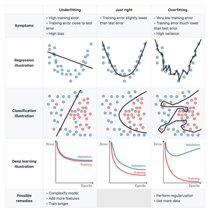
The Loss Curve (Train vs. Val): If train/loss continues to drop but val/loss starts rising, the model is overfitting (learning the plots by heart rather than the general forest structure).
Metrics, e.g., R² Score (biomass regression), overall accuracy and mean per-class accuracy (tree species classification)

Example: Model predicts dominant species very well, rare species always wrong: Overall accuracy = 90%, Mean class accuracy = 45%

Hyperparameter Tuning with Weights and Biases

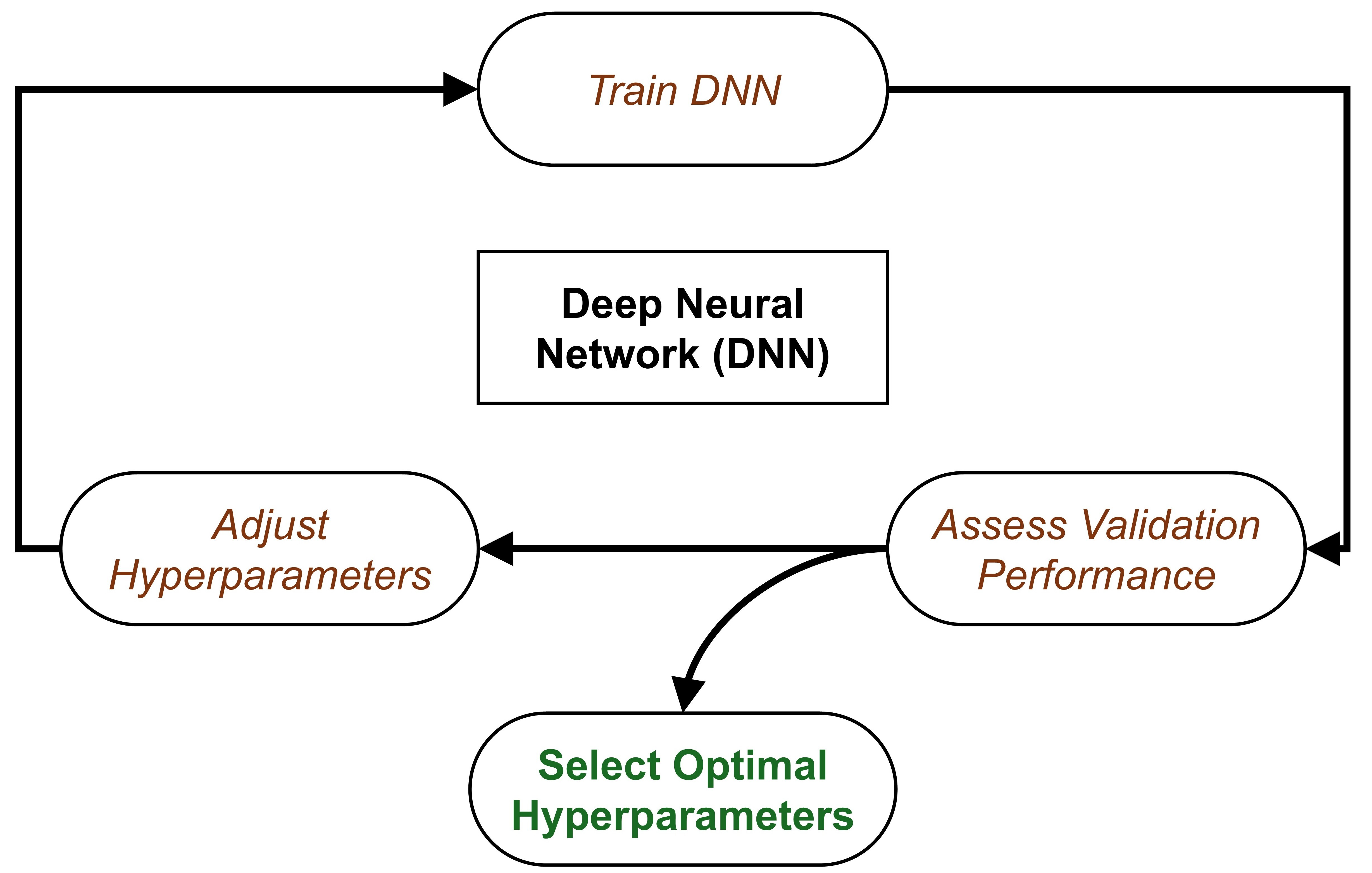
Compare results of different HPs using W&B Sweep: DGCNN example

Load Interactive W&B Sweep

Predicting (predict.py)

Once your model has finished hyperparameter tuning and you have selected the best checkpoint, you can run predictions. The output is saved as a CSV containing the ground truth and the model’s estimate.

Code

# predict.py
# ... same as training for configs loading, datamodule, modelmodule, trainer initialize
# 4. Run prediction
print("Running prediction...")
outputs = trainer.predict(model, dataloaders=data_module)

# 5. Parse outputs → CSV
records = []

if task == "classification":
    for o in outputs:
        for pid, gt, pred in zip(
            o["plot_id"],
            o["gt"],
            o["pred"]
        ):
            records.append({
                "plot_id": pid,
                "dom_sp_type": int(gt.item()),
                "pred_dom_sp_type": int(pred.item())
            })

else:  # regression
    for o in outputs:
        for pid, gt, pred in zip(
            o["plot_id"],
            o["gt"],
            o["pred"]
        ):
            records.append({
                "plot_id": pid,
                "total_agb_z": float(gt.item()),
                "total_agb_z_pred": float(pred.item())
            })

df = pd.DataFrame(records)
df.to_csv(os.path.join(os.path.dirname(args.ckpt_path), args.out_csv), index=False)

print(f"Predictions saved to: {os.path.join(os.path.dirname(args.ckpt_path), args.out_csv)}")

Tree Species Classification

For classification, we compare the categorical index of the dominant forest type between the ground truth and the model predictions. Table 2 shows the results of a DGCNN model classifying forest plots into type 0, 1, or 2 (Coniferous, Deciduous, Mixed).

Table 2: Example of Tree Species Classification Results

plot_id	dom_sp_type (Actual)	pred_dom_sp_type (Predicted)
PRF009	1	1
PRF076	0	0
PRF011	0	0
PRF122	2	2
PRF179	1	1

Biomass Regression

For regression, we compare the standardized Above Ground Biomass (AGB) values. This enables the calculation of quantitative performance metrics such as RMSE and the coefficient of determination (\(R^2\)). Table 3 provides example predictions.

Table 3: Example of Biomass Regression Results

plot_id	total_agb_z (Actual)	total_agb_z_pred (Predicted)
PRF009	-0.03388112783432007	-0.06726609170436859
PRF076	-0.342624306678772	-0.3901059031486511
PRF011	-0.22952325642108917	-0.29783695936203003
PRF122	0.3514338731765747	0.34753304719924927
PRF179	0.09915713965892792	1.4272195100784302

How to Run

Environment Setup

See the Get Started page.

Training

Classification

To train the DGCNN model on the Petawawa dataset for a species classification task:

python train_pl.py \
    --model dgcnn \
    --dataset_config_key petawawa_cls \
    --batch_size 16 \
    --epoch 150 \
    --learning_rate 0.0001 \
    --log_dir petawawa_species_cls_dgcnn \
    --process_data # First time / no cache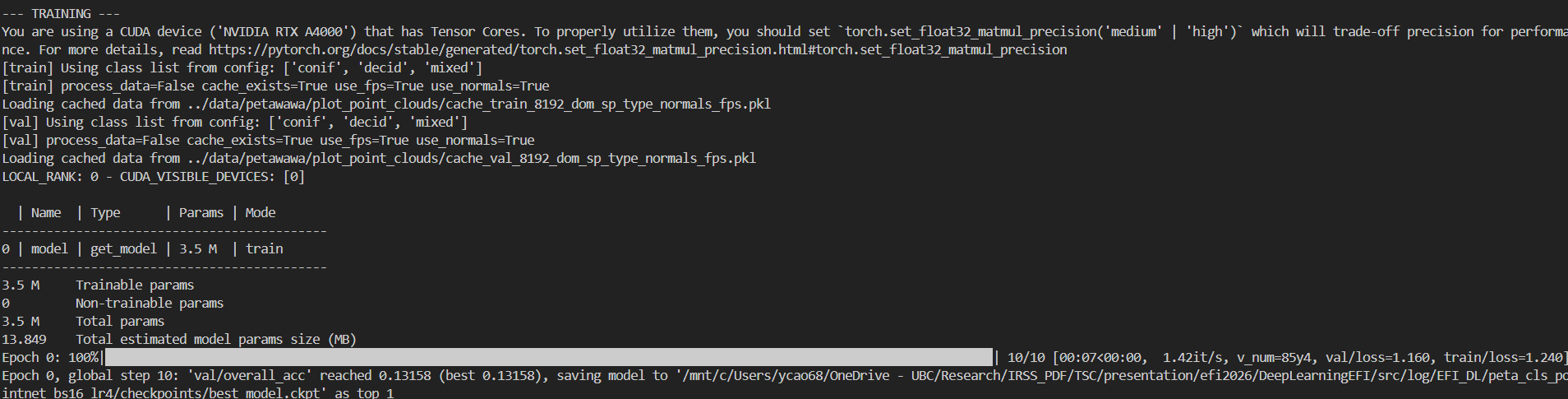

Regression

To train the DGCNN model on the Petawawa dataset for a biomass estimation task:

python train_pl.py \
    --model dgcnn \
    --dataset_config_key petawawa_reg \
    --batch_size 16 \
    --epoch 150 \
    --learning_rate 0.0001 \
    --log_dir petawawa_bio_reg_dgcnn \
    --process_data # First time / no cache

Testing

Classification

How to run:

wget -P /path/to/directory https://github.com/Brent-Murray/DeepLearningEFI/blob/main/src/pretrained_ckpt/peta_cls_dgcnn_bs16_lre4/checkpoints/best_model.ckpt 

python predict.py --model dgcnn --dataset_config_key petawawa_cls --ckpt_path /path/to/directory/best_model.ckpt

# example
python predict.py --model dgcnn --dataset_config_key petawawa_cls --ckpt_path log/EFI_DL/peta_cls_dgcnn_bs8_lre3/checkpoints/best_model.ckpt

Regression

How to run:

wget -P /path/to/directory https://github.com/Brent-Murray/DeepLearningEFI/blob/main/src/pretrained_ckpt/peta_reg_dgcnn_bs8_lre3/checkpoints/best_model.ckpt

python predict.py --model dgcnn --dataset_config_key petawawa_reg --ckpt_path /path/to/directory/best_model.ckpt

# example
python predict.py --model dgcnn --dataset_config_key petawawa_reg --ckpt_path log/EFI_DL/peta_reg_dgcnn_bs8_lre3/checkpoints/best_model.ckpt

Relevant Resources

Tutorial references of PyTorch Lightning

Paper

Code

Other Deep Learning Frameworks

Introduction

Deep Learning Pipeline

The Core Components of PyTorch Lightning:

The Data Foundation: The EFI Point Cloud Dataset

The EfiDataset (efi_dataset.py)

What it does

The EfiDataModule (efi_datamodule.py)

What it manages

The Model: EfiModelModule (efi_modelmodule.py)

How Dynamic Graph CNN (DGCNN) Works

Implement the DGCNN Model (dgcnn.py)

Loss Functions (loss_utils.py)

Evaluation Metrics (metrics.py)

Core components of the wrapper

Training Deep Learning Models in PyTorch Lightning

Configurations (config.py)

The PyTorch Lightning Trainer (train_pl.py)

Summary: EFI Deep Learning Pipeline Logic

Logic flow

Monitoring with Weights & Biases (W&B)

W&B Dashboard

What to Look for in the Dashboard

Hyperparameter Tuning with Weights and Biases

Predicting (predict.py)

Tree Species Classification

Biomass Regression

How to Run

Environment Setup

Training

Classification

Regression

Testing

Classification

Regression

The `EfiDataset` (efi_dataset.py)

The `EfiDataModule` (efi_datamodule.py)