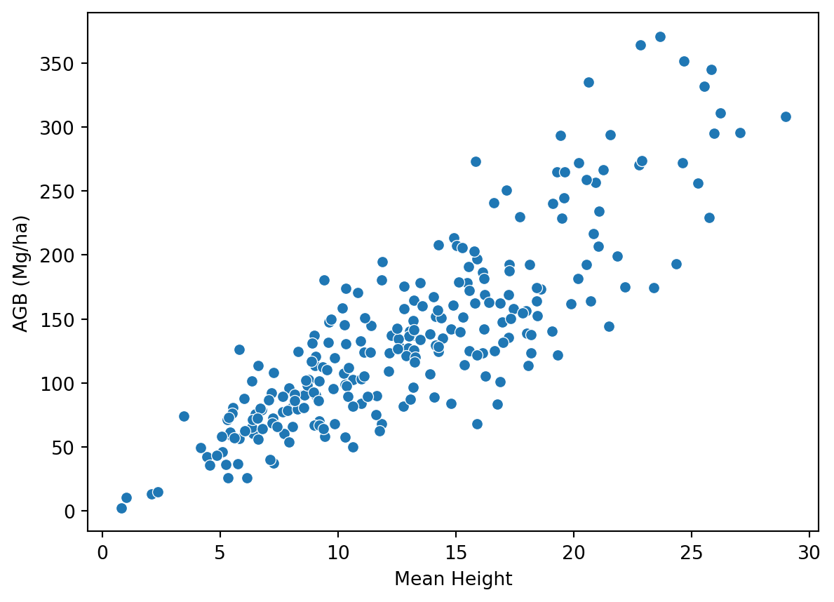
Deep Learning for Forest Inventories
  • Home
  • 1-Intro
  • 2-Data
  • 3-Train
  • 4-Evaluation
  • 5-Examples

On this page

  • Prepare data for RF Modelling
  • Train RF for Dominant Species Type Classification
  • Train RF for AGB estimation
  • Report an issue

Random Forest

This notebook trains random forest (RF) models to classify dominant tree species type and regress forest AGB using LiDAR metrics.

LiDAR metrics were calculated using the code below:

LiDAR Metric Derivation

Load packages

Code
import pandas as pd
import seaborn as sns
import numpy as np
import matplotlib.pyplot as plt
import geopandas as gpd
from sklearn.ensemble import RandomForestClassifier, RandomForestRegressor
from sklearn.metrics import accuracy_score, cohen_kappa_score, confusion_matrix, mean_squared_error, r2_score
import rioxarray as rio

from src.utils.regression_utils import plot_regression

Set filepaths

LABELS_FPATH = r'data/petawawa/labels.csv'

METRICS_FPATH = r'data/petawawa/lidar_metrics.csv'

Load labels and LiDAR metrics

metrics_df = pd.read_csv(METRICS_FPATH)

metric_names = metrics_df.drop('plot_id', axis=1).columns.tolist()

df = (pd.read_csv(LABELS_FPATH)
        .merge(metrics_df, on="plot_id", how='left')
        .rename(columns={'total_agb_mg_ha': 'agb_mg_ha_obs'})
        )

# View relationship between mean height and biomass
ax = sns.scatterplot(df, y='agb_mg_ha_obs', x='zmean')
ax.set(xlabel='Mean Height', ylabel='AGB (Mg/ha)')

Prepare data for RF Modelling

# Check which ALS metric cols have NAs
na_counts = df.isna().sum()

# Print all cols with NAs
for col, na_count in na_counts.items():
    if na_count > 0:
        print(f"{col}: {na_count} NAs")

# Drop rows with any NAs
df = df.dropna()
df
plot_id dom_sp_type perc_decid agb_mg_ha_obs split total_agb_z n zmax zmin zmean ... vzsd vzcv OpenGapSpace ClosedGapSpace Euphotic Oligophotic kde_peaks_count kde_peak1_elev kde_peak1_value HOME
0 PRF013 conif 0.000000 42.263648 train -1.326847 19533 12.11 -0.46 4.449033 ... 0.339932 86.693595 48.448852 24.437781 19.086611 8.026756 1 4.310411 0.149233 12.11
1 PRF090 mixed 52.285188 127.743892 train -0.130919 37466 29.91 -0.50 12.639579 ... 0.350017 107.110615 38.931903 43.288246 12.285448 5.494403 3 27.776575 0.009072 29.91
2 PRF015 conif 5.186690 172.347008 train 0.493109 18859 30.50 -0.75 15.571104 ... 0.198087 77.504066 32.883558 49.915951 10.412975 6.787515 3 22.196184 0.062241 30.50
3 PRF146 conif 3.228891 174.069178 train 0.517204 17623 33.47 -0.34 10.340951 ... 0.174707 179.575843 53.155319 36.181278 6.507298 4.156105 3 29.429452 0.043175 33.47
4 PRF208R conif 0.000000 13.298206 train -1.732093 20061 5.60 -0.14 2.092026 ... 0.389900 76.030501 37.703165 13.280582 25.684346 23.331908 1 2.157182 0.163660 5.60
... ... ... ... ... ... ... ... ... ... ... ... ... ... ... ... ... ... ... ... ... ...
244 PRF212 conif 26.719682 141.950651 test 0.067843 17128 32.35 -0.45 16.189422 ... 0.191256 76.990694 35.943012 48.303935 10.384441 5.368611 2 18.623973 0.058992 32.35
245 PRF049 mixed 66.054144 36.550006 test -1.406785 19089 18.85 0.00 5.244531 ... 0.243248 128.427960 58.916293 23.871450 10.014948 7.197309 2 13.318982 0.035563 18.85
246 PRF161 decid 98.688073 131.689708 test -0.075714 17089 23.53 -0.16 17.017618 ... 0.334060 133.360794 21.892537 62.961194 14.095522 1.050746 2 17.447084 0.134810 23.53
247 PRF199 conif 5.880717 133.009047 test -0.057256 58565 27.82 -0.38 10.962897 ... 0.192104 136.609411 40.449952 41.689097 11.096440 6.764512 3 20.052877 0.061518 27.82
248 PRF072 mixed 54.907966 65.969887 test -0.995180 17283 21.11 -0.15 7.421538 ... 0.362311 84.959235 50.054600 26.167076 13.452088 10.326235 1 7.062877 0.096511 21.11

249 rows × 102 columns

# Assign nummieric IDs to each dominant species
df['dom_sp_type_id'] = df['dom_sp_type'].astype('category').cat.codes

# Create a dictionary mapping species names to their IDs
dom_sp_dict = (df[['dom_sp_type', 'dom_sp_type_id']]
               .drop_duplicates()
               .sort_values(by='dom_sp_type_id')
               .set_index('dom_sp_type_id', drop=True)
               .to_dict()['dom_sp_type'])

dom_sp_dict
{0: 'conif', 1: 'decid', 2: 'mixed'}
train_df = df[df['split'] == 'train'].reset_index(drop=True)
test_df = df[df['split'].isin(('val', 'test'))].reset_index(drop=True)

train_df.columns
Index(['plot_id', 'dom_sp_type', 'perc_decid', 'agb_mg_ha_obs', 'split',
       'total_agb_z', 'n', 'zmax', 'zmin', 'zmean',
       ...
       'vzcv', 'OpenGapSpace', 'ClosedGapSpace', 'Euphotic', 'Oligophotic',
       'kde_peaks_count', 'kde_peak1_elev', 'kde_peak1_value', 'HOME',
       'dom_sp_type_id'],
      dtype='object', length=103)
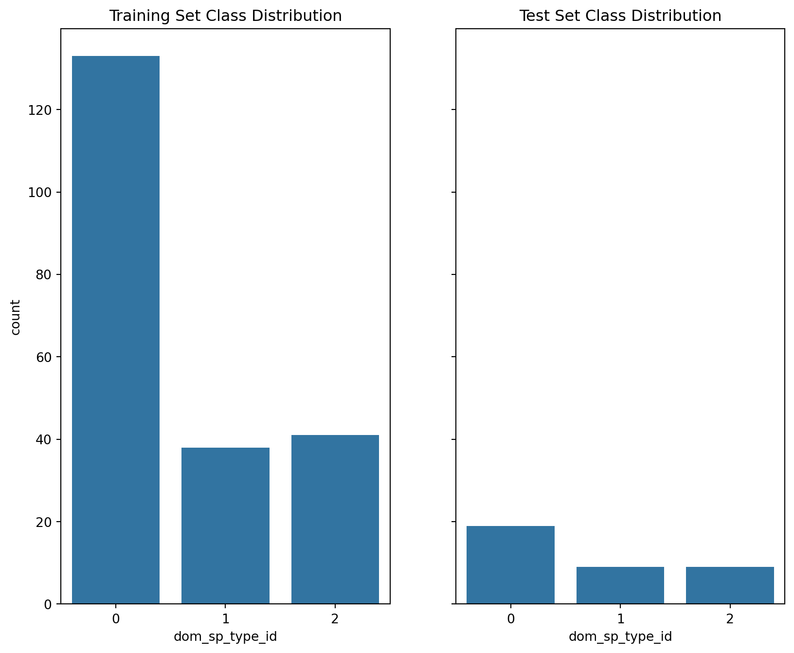
# Split data into train and test sets (combine val into test since not needed as seperate for RF)
train_df = df[df['split'].isin(('train', 'val'))].reset_index(drop=True)
test_df = df[df['split'] == 'test'].reset_index(drop=True)

# Create histograms showing each dataset class distributions
fig, axes = plt.subplots(1, 2, figsize=(10, 8), sharey=True)
sns.countplot(x='dom_sp_type_id', data=train_df, ax=axes[0])
axes[0].set_title('Training Set Class Distribution')
sns.countplot(x='dom_sp_type_id', data=test_df, ax=axes[1])
axes[1].set_title('Test Set Class Distribution')


plt.show()

Train RF for Dominant Species Type Classification

def plot_feature_importance(rf, metric_names, title):
    importances = rf.feature_importances_
    importance_df = pd.DataFrame({'Metric': metric_names, 'importance': importances
                                    }).sort_values(by='importance', ascending=False)
    plt.figure(figsize=(10, 6))
    sns.barplot(x='importance', y='Metric', hue='importance', data=importance_df, palette='viridis', legend=False)
    plt.title(title)
    plt.yticks(fontsize=5)
    plt.xlabel('Importance Score')
    plt.show()
rf = RandomForestClassifier(n_estimators=100, random_state=25)

rf.fit(train_df[metric_names], train_df['dom_sp_type_id'])

# Apply the model to the test set
test_df['pred_dom_sp_group_id'] = rf.predict(test_df[metric_names])

# Calculate accuracy and kappa
accuracy = accuracy_score(test_df['dom_sp_type_id'], test_df['pred_dom_sp_group_id'])
kappa = cohen_kappa_score(test_df['dom_sp_type_id'], test_df['pred_dom_sp_group_id'])

print(f"Overall Accuracy: {accuracy:.2f}")
print(f"Kappa: {kappa:.2f}")

# Class specific accuracies
class_accuracies = {}
for class_id in test_df['dom_sp_type_id'].unique():
    class_mask = test_df['dom_sp_type_id'] == class_id
    class_accuracy = accuracy_score(test_df.loc[class_mask, 'dom_sp_type_id'],
                                    test_df.loc[class_mask, 'pred_dom_sp_group_id'])
    class_accuracies[class_id] = class_accuracy
    print(f"Class {class_id} ({dom_sp_dict[class_id]}): Accuracy = {class_accuracy:.2f}")


# Print confusion matrix
conf_matrix = confusion_matrix(test_df['dom_sp_type_id'], test_df['pred_dom_sp_group_id'])

fig, ax = plt.subplots(figsize=(6,5), layout='tight')

sns.heatmap(ax=ax, data=conf_matrix, annot=True, fmt='d', cmap='Blues',
            xticklabels=dom_sp_dict.values(),
            yticklabels=dom_sp_dict.values())

ax.set_xlabel('Predicted Label')
ax.set_ylabel('Observed Label')
ax.set_title('Random Forest', fontsize=14, fontweight='bold')

fig.savefig("images/rf_cls_confusion_matrix.jpg", dpi=300)

# View metric importance
plot_feature_importance(rf, metric_names, title='Feature Importance from Random Forest Classifier')
Overall Accuracy: 0.76
Kappa: 0.57
Class 1 (decid): Accuracy = 0.67
Class 0 (conif): Accuracy = 0.95
Class 2 (mixed): Accuracy = 0.44

Train RF for AGB estimation

rf = RandomForestRegressor(n_estimators=100, random_state=25)

rf.fit(train_df[metric_names], train_df['agb_mg_ha_obs'])

test_df['agb_mg_ha_pred'] = rf.predict(test_df[metric_names])

# Plot regression results
plot_regression(obs=test_df['agb_mg_ha_obs'], 
                pred=test_df['agb_mg_ha_pred'],
                title='Random Forest',
                ax_lims=(0, 400),
                fig_out_fpath='images/rf_regression_plot.jpg')

plot_feature_importance(rf, metric_names, title='Feature Importance from Random Forest Regressor')

  • Report an issue